
Findings F97 Plants, trees and earth, Biology and medicine found 2026-10-29
Tree rings track the broad drought pattern in a gridded record and almost none of its local detail
Across 664 western North American tree-ring sites, the trees pass almost none of the summer drought signal at scales below about 55 km and most of it above about 460 km, measured against a gridded climate record. That grid is itself smoothed over hundreds of kilometres, so part of the missing fine detail may belong to the grid and not to the trees. Three further tests on how drought moves through space and time came back null.
- Tier
- B*, strong signal
- Outcome
- mixed
- Rung
- hypothesis
- Verdicts
- 5 passed, 6 failed
- Corrections
- 2, latest 2026-11-14
- Version
- v3, 2026-11-14
- Redo it
- Reproduce
Download PDF 602 KB BuildTeX source F97.bld
What this means for a reader
A tree-ring site that matches its local drought record only weakly is not a weak drought recorder in every sense. In the American West the trees carry most of the broad, regional pattern of summer drought and almost none of the local detail, as far as a gridded record that is itself smoothed can show. When a proxy is scored site by site, ask how much of its lost skill is lost in space rather than in time.
Objection
CRU interpolates precipitation with a 450 km decay distance, right where the filter opens, so low fine-scale coherence may be smoothing in the reference. Site clustering and noise fill the finest band.
What would change the call. Repeat with station or denser gridded data as reference, another region, a held-out fine-scale network.
From the strongest objection recorded in our publication register.
Abstract
Tree-ring records are often judged one site at a time, by comparing a site's yearly growth with the climate at that spot. We split that comparison by spatial scale as well as by time scale. The data are June to August drought from a gridded index, 399 one-degree cells in western North America from 1903 to 2025, and 664 tree-ring chronologies in the same box, complete from 1903 to 1980. In each of 30 cells of a grid of six spatial bands and five time bands we measured the share of the drought signal that the trees pass. The preregistered contrast between broad, slow scales and fine, fast scales was 0.64 (95% interval 0.62 to 0.68), against 95th percentiles of 0.22 for phase-randomised trees and 0.30 for trees moved to shuffled sites, with an adjusted p of 0.035. Below 55 km the trees pass at most 0.004 of the drought signal in every time band, and above 460 km they pass 0.27 to 0.91. Three tests on the drought field came back null. The drought field's covariance did not depart from a space part times a time part, no travel speed could be claimed, and broad and fine patterns lose their memory at the same rate, with a dispersion exponent of 0.02 (-0.12 to 0.17). Measured against this gridded record, the trees act as a spatial filter; the grid is itself smooth, so the filter may belong partly to the grid.
c1 observed, evidence for claim 1
- The numbers in claim 1
- 0.64; 95; 0.62; 0.68; 0.22; 0.30; 0.035 matches the result file, 2026-11-09
- Chart 2
- The tree filter's contrast against its two controls.
- Basis
- observed: measured in this study, with a result file
c2 observed, evidence for claim 2
- The numbers in claim 2
- 55; 0.004; 460; 0.27; 0.91 matches the result file, 2026-11-09
- Chart 3
- Share of the drought signal the trees pass, by space scale and time scale.
- Chart 4
- Where the variance sits: tree rings against the drought index at the same sites.
- Basis
- observed: measured in this study, with a result file
c3 observed, evidence for claim 3
- Basis
- observed: measured in this study, with a result file
- Numbers
- None in the sentence; it reads the numbers stated beside it.
c4 observed, evidence for claim 4
- Basis
- observed: measured in this study, with a result file
- Numbers
- None in the sentence; it reads the numbers stated beside it.
c5 observed, evidence for claim 5
- The numbers in claim 5
- 0.02; -0.12; 0.17 matches the result file, 2026-11-09
- Chart 5
- Dispersion exponent of the drought field against the planted fields.
- Basis
- observed: measured in this study, with a result file
Introduction
Tree rings are the main yearly record of drought before instruments. Cook, Meko, Stahle and Cleaveland [1] built a grid of summer drought reconstructions for the United States from a dense network of chronologies. Their method fits each grid point from the chronologies within a search radius, and they reported that a radius of 450 km worked best. The method is local by design. The reconstructed maps still kept the spatial features of drought, which the authors noted although the method was not built to be spatial.
The drought index in this study is the self-calibrating Palmer Drought Severity IndexDefinition: self-calibrating Palmer Drought Severity Index (scPDSI) climatology and hydrology A monthly drought index computed from temperature and precipitation through a simple soil water balance, with its constants calibrated to each location so values compare across places. Excludes a direct measurement of soil moisture or of streamflow. full definition, the scPDSI. Wells, Goddard and Hayes [2] built it so that the index's constants are fitted to each location and values compare across places. We use the gridded scPDSI distributed with CRU TS 4.10 [3] [4].
Averaging trees over larger areas raises the shared climate signal. Duchesne and colleagues [6] showed with forest inventory cores in Quebec that averaging at the stand level removes tree-level noise, that covariance among tree-ring signals falls with distance, and that reliable climate signals can be drawn at scales from 37 to 583,000 square km.
These studies treat space and time one at a time. A field that varies in both can hold structure neither view shows: a front that moves, patterns that fade faster at fine scales than at broad ones, or a filter that passes some combinations of scale and period and not others. This paper asks four questions at once. Does the drought field's covariance split into a space part times a time part? Do its anomalies travel? Do broad and fine patterns fade at different rates? And which combinations of spatial scale and period do the tree rings pass?
Preregistration and design
The design was written and hash-locked on 30 October 2026 at 04:20 UTC as a preregistrationDefinition: preregistration research method (metascience) A dated written plan for a study, fixed and hash-locked before any result is seen: the question, the data, the statistic, the controls, the forecasts and the kill conditions. Excludes a plan revised after looking at the outcome, and a protocol written only for the record after the run. full definition, before any outcome on the real data was computed. The real data had been built and only their counts printed: 399 cells by 123 years and 664 sites by 78 years. Development before the lock used synthetic fields only, and the preregistration lists every change made during that development.
The locked file names the data, the band edges, the four statistics, the synthetic fields, each controlDefinition: control statistics and experimental design A version of the data with the structure under test removed (for example shuffled or pooled), scored the same way as the real data, so the real score has something to beat. Excludes a comparison with a different dataset or with a published number. full definition, the forecasts and the pass rules. No unit, constant or rule changed after the lock. Each test passes only when the real statistic beats the 95th percentile of every scoring control, its adjusted p value is 0.05 or less, and, where named, its bootstrap interval sits above 0. A test that misses any rule fails, which makes each rule a kill conditionDefinition: kill condition research method (our usage, after Popper's falsification) A rule written in the preregistration that, when met, decides against the claim with no room for judgement after the run. Excludes reasons found after the run for setting a result aside. full definition.
Forecasts, written before the run: the covariance would be non-separable in both fields; travel would most likely be null or slow, under 100 km per year; the dispersion exponent would lie between 0 and 2, closer to the diffusion reading than the wave reading; and the tree filter test would pass.
Data and provenance
Drought: the June to August mean of the scPDSI from CRU TS 4.10 [4], 0.5 degree, 1903 to 2025, released under the Open Database License 1.0. The 0.5 degree cells between 125 and 100 W and 30 and 50 N were averaged to one-degree cells, keeping only one-degree cells with all four parts present in every year. This gave 399 cells and 123 years.
Trees: standard ring-width chronologiesDefinition: tree-ring chronology dendrochronology One yearly series for a site, built by dating many cores, removing each core's age and size trend and averaging the results into a dimensionless index. Excludes a single core's raw ring widths, and a climate reconstruction made from the series. full definition from the International Tree-Ring Data Bank [5], held by NOAA's National Centers for Environmental Information as public data, with a request to cite the contributors. Every site in the same box with a gap-free index from 1903 to 1980 entered, which gave 664 sites and 78 years. Each site was paired with the June to August scPDSI of its nearest 0.5 degree cell with data in every year.
Every series had its linear trend removed and was scaled to unit variance. Positions were projected about 112.5 W and 40 N, in km. The input files and code were hashed into the run record before the run.
Methods
Bands in space and time
Let be the matrix that smooths values on the sites with a normalised Gaussian of width , where to are 55, 95, 160, 270 and 460 km. Set to the identity and to zero. The space bandDefinition: space band signal processing on irregular sites, our usage The part of a field that varies between two spatial scales, taken as the difference of two Gaussian smoothings of the site values with the two scales as widths. The six bands add back to the field. Excludes an exact wavenumber, because the bands overlap and the sites are irregular. full definition of a field is
for from 0 to 5, so band 0 holds what varies below about 55 km and band 5 what varies above about 460 km, and the six bands add back to . Each band is then split into five time bandsDefinition: time band spectral analysis The part of a yearly series whose period lies between two limits, kept by masking its Fourier transform. Excludes a moving average or a fitted trend. full definition by masks on the Fourier transform in time with edges at 1/32, 1/16, 1/8 and 1/4 cycles per year: periods over 32 years, 16 to 32, 8 to 16, 4 to 8 and 2 to 4 years. Each masked series is kept as a complex analytic signal.
The tree filter
For space band and time band , let and be the analytic signals of drought at the tree sites and of the trees. Summing over sites and years, with the sum of and , the sums of squared magnitudes, the passed share is the squared coherenceDefinition: squared coherence spectral analysis The share of one series' variance in a frequency band that a linear filter of the other series can account for, between 0 and 1. Here pooled over sites and years in each space and time band and called the passed share. Excludes a nonlinear dependence, and the size of the response, which the gain measures. full definition
The preregistered contrast is the mean of over the four broad, slow cells (space bands 4 and 5, periods over 16 years) minus its mean over the four fine, fast cells (space bands 0 and 1, periods under 8 years):
where and name those two sets of cells.
Separability
Let be the correlation between sites at distance and time lag , pooled over pairs in 100 km bins to 800 km and lags of 1, 2 and 3 years. A separable covarianceDefinition: separable covariance space-time statistics A covariance that factors into a function of distance times a function of time lag, so the spatial pattern of correlation has the same shape at every lag. Excludes fields whose anomalies travel or whose broad and fine patterns fade at different rates. full definition has . With fitted by least squares, the statistic is the sum of squared departures
Travel
For site pairs within 1,200 km, the lag-one cross-correlation between site in one year and site in the next is pooled in 40 km offset cells and fitted as
where is the offset between the sites, the lag-zero correlation profile by distance, a scale and a velocity in km per year.
Dispersion
The decay rate of a pattern with wavenumber is modelled as , with power per log wavenumber proportional to and white site noise. Each interior space band's autocovariance at lags 0 to 8 is predicted from the measured transfer of plane waves through that band on these exact sites and from the bias that linear detrending adds, and the four parameters are fitted to bands 1 to 4. The dispersion exponentDefinition: dispersion exponent physics of waves and diffusion The power beta in a decay rate that grows as the wavenumber to the power beta. Diffusion gives about 2, and fine and broad patterns that fade at the same rate give 0. Excludes a speed of travel, which the propagation test measures. full definition is the result. Beside it, each band's e-folding time is reported.
p values, intervals and multiplicity
Each control was drawn 200 times, or 300 times for the separable surrogate. A test's p value is the larger of its scoring controls' p values from drawsDefinition: p value (from draws) statistics The share of control draws scoring at or above the real score, with one added to the count and to the number of draws, so it is never zero. Excludes a p value from a textbook formula that assumes a distribution. full definition,
with the draws at or above the real value and the draws. The seven real-data tests were adjusted together with the Benjamini-Hochberg correctionDefinition: Benjamini-Hochberg correction statistics, multiple testing A rule that adjusts a set of p values so that, among the tests called significant, the expected share of false calls stays at or below a chosen rate q, here 0.05. Excludes the stricter Bonferroni rule, which bounds the chance of any false call. full definition at q 0.05. Every 95% intervalDefinition: 95% interval statistics The range that holds the middle 95 percent of the bootstrap or control draws for a number. We report it beside the number. Excludes a statement that the true value lies inside with 95 percent probability. full definition comes from a moving-block bootstrapDefinition: moving-block bootstrap statistics An interval made by recomputing a statistic many times on years resampled in runs of consecutive years, here 10, so that year-to-year correlation is kept inside each run. Excludes resampling single years as if they were independent. full definition in time with blocks of 10 years.
Controls and planted checks
A planted checkDefinition: planted check research method; called a positive control in experimental science Data built so that the right answer is known, run through the same analysis before the real data, to show that the analysis can see the effect when it is there. Excludes any check made on the real data, which cannot show what the analysis misses. full definition ran in the same job before the real data were scored. Synthetic fields were built on the drought cell positions with 123 years, from 800 random plane waves plus white noise: a separable field, a wave field carried at 120 km per year toward 30 degrees, a diffusing field and pure noise. Five realisations of each were scored, and the instrument passed every rule. The separable field read as separable (median p 0.37 against a rule of at least 0.05), the planted wave's speed came back within 2.2 percent and its direction within 0.66 degrees, and the diffusion exponent read 1.88 against a rule of 1.7 to 2.3. On the separable field the exponent read -0.01 and on the wave 0.81. Those are the readings a real exponent is compared against. The same checks on the tree positions with 78 years were reported and not scored; there the diffusion exponent read 1.64, below the scoring range.
c6 observed, evidence for claim 6
- The numbers in claim 6
- 0.37; 0.05; 2.2; 0.66; 1.88; 1.7; 2.3 matches the result file, 2026-11-09
- Chart 1
- The design: one instrument, checked on planted fields, then four questions put to real drought and tree rings.
- Basis
- observed: measured in this study, with a result file
- dataSummer drought index and tree rings399 drought cells over 123 years and 664 ring-width sites over 78 years, western North America.
- planted checkPlanted fields with known answersA field that is a space part times a time part read as such (median p 0.37). A planted wave's speed came back within 2.2 percent. A planted diffusing field read 1.88 against a true 2.
- measurementThree questions on the drought fieldDoes its covariance depart from space times time? Does it travel? Do broad patterns outlast fine ones?
- measurementOne question on the treesWhich space and time scales of drought do tree rings pass? The contrast is the passed share at broad, slow scales minus the share at fine, fast scales.
- controlControls drawn 200 to 300 timesShuffled site positions, phase-randomised series (each site keeps its spectrum, timing scrambled) and a fitted separable field.
- rule set in advanceRule: beat every control's 95th percentileWith p adjusted over all seven real-data tests below 0.05.
- three nullsDrought field: separability, travel, dispersionAdjusted p 0.91, 0.66 and 0.80.
- passedTree filterContrast 0.64, adjusted p 0.035.
Read from result.json, run 20261030T042024Z. SHA-256 of the run's file 6d1917adb4c50b78125146ee5dcaa42c6081a05edc4bcb1920e72fbc3b60cf0d and of the published copy a28f36d4828f91a94e8b319efdd8484124222e281175fdd885acf21a3ffb1891. In the copy, file paths are cut to the file name and the layout (indentation, line endings) may differ; every value is the same.
The real statistics faced these controls, each drawn many times to give a null distributionDefinition: null distribution statistics The spread of scores a control gives over many random draws. Its 95th percentile is the bar a real score must clear. Excludes a theoretical distribution assumed rather than drawn from the data. full definition. Separability: a fitted separable field with the same lag-zero spatial covariance and pooled time autocovariance, and shuffled site coordinates. Travel: the lag-one matrix with its symmetric part kept and its antisymmetric part permuted across pairs in 100 km distance bins, and shuffled coordinates. Dispersion: shuffled coordinates and phase randomisationDefinition: phase randomisation time-series statistics, surrogate data A copy of a series with the same power spectrum and random Fourier phases, so it keeps the series' autocorrelation and loses its timing against any other series. Excludes shuffling years, which also destroys the autocorrelation. full definition of each site. The tree filter: phase-randomised trees, and tree series reassigned to shuffled sites. The last control keeps every tree's own spectrum and breaks only the link to its place.
Results
The tree filter
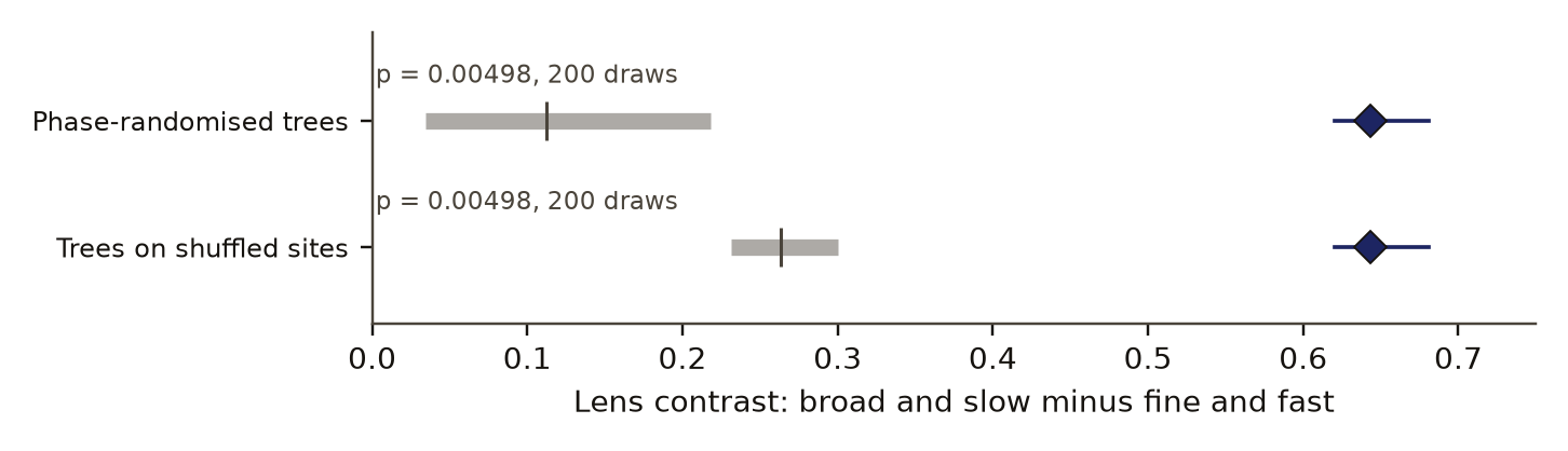
The preregistered contrast between broad, slow scales and fine, fast scales was 0.64 (95% interval 0.62 to 0.68), against 95th percentiles of 0.22 for phase-randomised trees and 0.30 for trees moved to shuffled sites, with an adjusted p of 0.035. Figure 1 sets the contrast against both controls.
contrast (higher: broad, slow drought passes better)
- measured contrast
- control, 5th to 95th percentile
- control mean
Data behind chart 2 3 rows
| Quantity | Value | 5th percentile | Mean | 95th percentile | p |
|---|---|---|---|---|---|
| Measured contrast | 0.643 | 0.620 (interval low) | 0.681 (interval high) | 0.005, adjusted 0.035 | |
| Phase-randomised trees | 0.034 | 0.112 | 0.218 | 0.005 | |
| Trees at shuffled sites | 0.232 | 0.263 | 0.300 | 0.005 |
Read from result.json, run 20261030T042024Z. SHA-256 of the run's file 6d1917adb4c50b78125146ee5dcaa42c6081a05edc4bcb1920e72fbc3b60cf0d and of the published copy a28f36d4828f91a94e8b319efdd8484124222e281175fdd885acf21a3ffb1891. In the copy, file paths are cut to the file name and the layout (indentation, line endings) may differ; every value is the same.
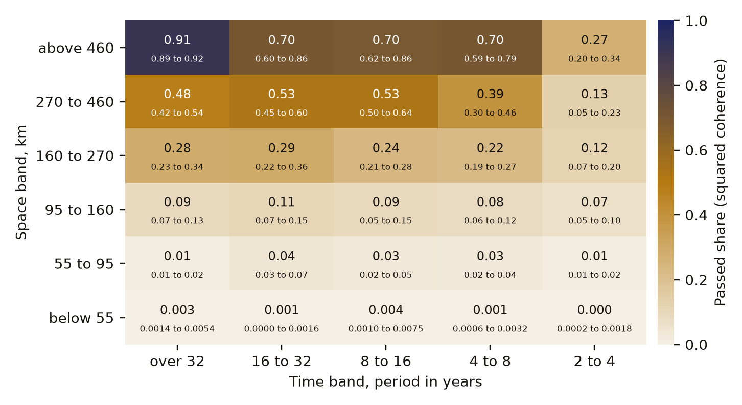
Figure 2 gives the passed share in all 30 cells. The share rises with spatial scale in every time band. Below 55 km the trees pass at most 0.004 of the drought signal in every time band, and above 460 km they pass 0.27 to 0.91. Between 95 and 160 km they pass 0.07 to 0.11, and between 270 and 460 km 0.13 to 0.53. Time scale matters most at the broad end: above 460 km the share is 0.91 at periods over 32 years and 0.27 at 2 to 4 years. The phase-randomised control's mean share is at most 0.18, in that broadest and slowest cell.
| Space scale \ period | over 32 years | 16 to 32 years | 8 to 16 years | 4 to 8 years | 2 to 4 years |
|---|---|---|---|---|---|
| below 55 km | 0.003 | 0.0005 | 0.004 | 0.001 | 0.0005 |
| 55 to 95 km | 0.015 | 0.043 | 0.032 | 0.028 | 0.015 |
| 95 to 160 km | 0.094 | 0.11 | 0.094 | 0.083 | 0.065 |
| 160 to 270 km | 0.28 | 0.29 | 0.24 | 0.22 | 0.12 |
| 270 to 460 km | 0.48 | 0.53 | 0.53 | 0.39 | 0.13 |
| above 460 km | 0.91 | 0.70 | 0.70 | 0.70 | 0.27 |
Data behind chart 3 30 rows
| Space scale | Period | Passed share | Interval low | Interval high |
|---|---|---|---|---|
| below 55 km | over 32 years | 0.0034 | 0.0014 | 0.0054 |
| below 55 km | 16 to 32 years | 0.0005 | 0.0000 | 0.0016 |
| below 55 km | 8 to 16 years | 0.0038 | 0.0010 | 0.0075 |
| below 55 km | 4 to 8 years | 0.0012 | 0.0006 | 0.0032 |
| below 55 km | 2 to 4 years | 0.0005 | 0.0002 | 0.0018 |
| 55 to 95 km | over 32 years | 0.0146 | 0.0108 | 0.0243 |
| 55 to 95 km | 16 to 32 years | 0.0427 | 0.0252 | 0.0675 |
| 55 to 95 km | 8 to 16 years | 0.0320 | 0.0167 | 0.0518 |
| 55 to 95 km | 4 to 8 years | 0.0283 | 0.0233 | 0.0394 |
| 55 to 95 km | 2 to 4 years | 0.0147 | 0.0088 | 0.0220 |
| 95 to 160 km | over 32 years | 0.0937 | 0.0720 | 0.1277 |
| 95 to 160 km | 16 to 32 years | 0.1059 | 0.0685 | 0.1468 |
| 95 to 160 km | 8 to 16 years | 0.0941 | 0.0541 | 0.1472 |
| 95 to 160 km | 4 to 8 years | 0.0826 | 0.0628 | 0.1237 |
| 95 to 160 km | 2 to 4 years | 0.0651 | 0.0457 | 0.0968 |
| 160 to 270 km | over 32 years | 0.2828 | 0.2313 | 0.3431 |
| 160 to 270 km | 16 to 32 years | 0.2892 | 0.2183 | 0.3596 |
| 160 to 270 km | 8 to 16 years | 0.2377 | 0.2055 | 0.2821 |
| 160 to 270 km | 4 to 8 years | 0.2246 | 0.1916 | 0.2680 |
| 160 to 270 km | 2 to 4 years | 0.1182 | 0.0681 | 0.2035 |
| 270 to 460 km | over 32 years | 0.4805 | 0.4219 | 0.5435 |
| 270 to 460 km | 16 to 32 years | 0.5297 | 0.4522 | 0.5992 |
| 270 to 460 km | 8 to 16 years | 0.5284 | 0.4957 | 0.6383 |
| 270 to 460 km | 4 to 8 years | 0.3915 | 0.3029 | 0.4573 |
| 270 to 460 km | 2 to 4 years | 0.1324 | 0.0451 | 0.2281 |
| above 460 km | over 32 years | 0.9059 | 0.8873 | 0.9236 |
| above 460 km | 16 to 32 years | 0.7023 | 0.5970 | 0.8593 |
| above 460 km | 8 to 16 years | 0.6952 | 0.6235 | 0.8597 |
| above 460 km | 4 to 8 years | 0.7009 | 0.5872 | 0.7888 |
| above 460 km | 2 to 4 years | 0.2663 | 0.2014 | 0.3407 |
Read from result.json, run 20261030T042024Z. SHA-256 of the run's file 6d1917adb4c50b78125146ee5dcaa42c6081a05edc4bcb1920e72fbc3b60cf0d and of the published copy a28f36d4828f91a94e8b319efdd8484124222e281175fdd885acf21a3ffb1891. In the copy, file paths are cut to the file name and the layout (indentation, line endings) may differ; every value is the same.
share of variance
- tree rings
- drought index at the tree sites
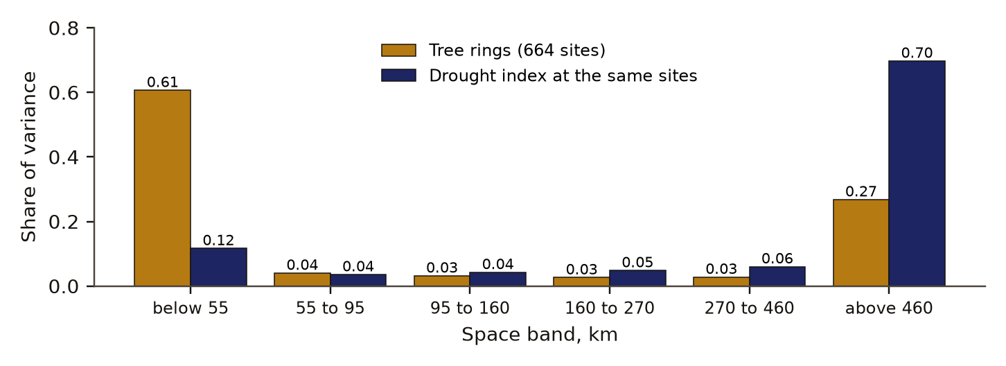
Data behind chart 4 6 rows
| Space scale | Tree rings | Drought index at the tree sites |
|---|---|---|
| below 55 km | 0.607 | 0.117 |
| 55 to 95 km | 0.040 | 0.036 |
| 95 to 160 km | 0.032 | 0.043 |
| 160 to 270 km | 0.026 | 0.048 |
| 270 to 460 km | 0.028 | 0.060 |
| above 460 km | 0.268 | 0.697 |
Read from spacetime-panel.json. SHA-256 of the run's file 8dfd9b181155952b5d29748aa73dd8de0166689a35618eeecc0f6293a2652531, published unchanged.
The trees' own variance sits where their filter is closed. Figure 3 shows that 0.61 of the tree variance lies in the finest space band, against 0.12 for the drought index at the same sites.
The drought field
Table 1 gives all seven real-data tests. The drought field's covariance did not depart from a space part times a time part: its departure was 0.0011 against a separable-surrogate 95th percentile of 0.0085 (p 0.72). The trees came back the same way (p 0.35). Both fields beat shuffled coordinates, which only shows that nearby sites are alike.
The drought fit for travel pointed 34.5 degrees north of east at 64.5 km per year and beat the antisymmetric shuffle (95th percentile 32 km per year). It did not beat shuffled coordinates, whose 95th percentile was 467 km per year, and no travel speed could be claimed: the bootstrap interval of the speed along the fitted direction ran from -41 to 242 km per year and the adjusted p was 0.66.
Broad and fine patterns lose their memory at the same rate, with a dispersion exponent of 0.02 (-0.12 to 0.17). The e-folding times of the four interior bands were 0.76 to 0.83 years. Neither 1 nor 2 lies inside the interval, and the reading sits at the instrument's separable value, not at its wave or diffusion value. The trees' dispersion fit stopped at its lower bound of -1 and says nothing.
dispersion exponent
- drought index
- planted field, median of five
- 95% bootstrap interval of the drought exponent
- 1, a travelling wave
- 2, diffusion
Data behind chart 5 7 rows
| Field | Exponent | Interval low | Interval high |
|---|---|---|---|
| Drought index | 0.019 | −0.124 | 0.166 |
| Tree rings (fit at its lower bound) | −1.0 | −1.0 | 0.909 |
| Planted separable field, median | −0.013 | ||
| Planted wave, median | 0.812 | ||
| Planted diffusion, median | 1.876 | ||
| Control, shuffled coordinates (5th, 95th) | −0.001 | −0.156 | 0.143 |
| Control, phase-randomised (5th, 95th) | 0.012 | −0.120 | 0.143 |
Read from result.json, run 20261030T042024Z. SHA-256 of the run's file 6d1917adb4c50b78125146ee5dcaa42c6081a05edc4bcb1920e72fbc3b60cf0d and of the published copy a28f36d4828f91a94e8b319efdd8484124222e281175fdd885acf21a3ffb1891. In the copy, file paths are cut to the file name and the layout (indentation, line endings) may differ; every value is the same.
Read from spacetime-panel.json. SHA-256 of the run's file 8dfd9b181155952b5d29748aa73dd8de0166689a35618eeecc0f6293a2652531, published unchanged.
Table 2 sets the forecasts against the outcomes.
Discussion
The tree-ring network behaves as a spatial filter. It passes most of the drought signal at scales of several hundred km and above and almost none below 55 km. A site-by-site comparison of rings and local drought averages over that whole range and reports one number, so it reads as a weak recorder. In our findings ledgerDefinition: findings ledger our records The append-only, dated list of every result we have recorded, numbered F1, F2 and on. Corrections are added as new dated lines and old entries are never rewritten. Excludes a curated list of successes. full definition, a site-by-site comparison in time only, run after the preregistered test as exploration, gave pooled coherence of 0.24, 0.18, 0.19, 0.20 and 0.07 across the five time bands: weak and nearly flat in period. The space-time view places the weakness in space.
The result agrees with two lines of earlier work. Cook and colleagues [1] found that chronologies within a radius of about 450 km predict a drought grid point best, which is the scale at which our filter opens. Duchesne and colleagues [6] found that averaging over stands removes tree-level noise and that the shared signal falls with distance. Our grid puts both on one map of scale and period, with a number and an interval in each cell.
The three nulls on the drought field matter in their own right. If the field had a travelling front or patterns that faded at scale-dependent rates, separate views in space and in time would miss them. Here they did not: at one-degree cells and yearly steps, the separate views lose nothing a coupled view could find. The coupling that matters lies in the tree filter. Each null is an honest nullDefinition: honest null research method (our usage) A working test that found no effect beyond a stated bound, a forecast that failed, or an error of our own found and fixed, reported with the same weight as a positive result. Excludes a void run, and a result left unpublished because it was negative. full definition from a working instrument, since the planted wave and the planted diffusion were each recovered.
Part of the filter may belong to the reference grid. Harris and colleagues [3] report that CRU interpolates precipitation with a correlation decay distance of about 450 km, close to where the filter opens, so a smooth reference would itself pass little fine-scale signal to agree with. The next study needs station data or a denser grid as the reference.
Limitations
- The drought grid is smooth by construction, so part of the low fine-scale coherence may come from the reference and not from the trees.
- Tree sites cluster, so the finest band partly reads site noise and how dense the network is.
- The nulls on travel and dispersion hold for summer scPDSI at one degree, yearly steps, a box about 2,000 km across and 1903 to 2025. Monthly data, a larger domain or another index could show more.
- The scPDSI is a model built from temperature and precipitation, not a measurement of soil water.
- The trees' dispersion fit stopped at its bound and tells us nothing. On the tree positions the planted diffusion read 1.64, below the scoring range; that check was reported, not scored.
- The site-by-site comparison in the discussion was exploratory and not preregistered.
- Scoring was done by our own code and was not blind.
Evidence
Mixed. The broad-against-fine contrast held: 0.64 against control 95th percentiles of 0.22 and 0.30. The three tests on the drought field itself, separability, travel and dispersion, came back null on the climate grid and on the trees, so six of the eleven preregistered verdicts failed.
Figures
These are the paper's own figures, numbered as in the PDF, and each "Figure" reference in the text points here. The charts on this page redraw the same results from the result files and carry their own numbers.
Tables
| Test | Estimate (95% interval) | Controls, 95th percentile | Adjusted p | Verdict |
|---|---|---|---|---|
| Separability, drought | D 0.0011 (0.0004 to 0.0125) | separable 0.0085; shuffled 0.00008 | 0.91 | fail |
| Separability, trees | D 0.0017 (0.0012 to 0.0063) | separable 0.0042; shuffled 0.00013 | 0.80 | fail |
| Travel, drought | 64.5 km per year; along direction -41 to 242 | antisymmetric 32; shuffled 467 | 0.66 | fail |
| Travel, trees | 8.3 km per year; along direction -185 to 401 | antisymmetric 14.6; shuffled 462 | 0.91 | fail |
| Dispersion, drought | beta 0.02 (-0.12 to 0.17) | shuffled 0.14; phase 0.14 | 0.80 | fail |
| Dispersion, trees | beta -1, at its bound (-1 to 0.91) | shuffled 3.5; phase 3.0 | 1.0 | fail |
| Tree filter contrast | 0.64 (0.62 to 0.68) | phase 0.22; shuffled sites 0.30 | 0.035 | pass |
| Question | Forecast | Outcome |
|---|---|---|
| Separability | non-separable in both fields | separable in both; forecast failed |
| Travel | most likely null or slow, under 100 km per year | null; held |
| Dispersion | beta between 0 and 2, nearer diffusion | 0.02, at the separable reading; partly held |
| Tree filter | pass | pass; held |
Appendix A. The preregistered verdicts
Each verdictDefinition: verdict research method (our usage) The pass or fail of one preregistered rule set against the run's numbers, read off by code. Excludes an interpretation written after reading the numbers. full definition is a set of rules written before the run, and it passes only when every rule holds. Values are read from the run's result file.
| Verdict | Deciding rule | Value | Holds |
|---|---|---|---|
| Instrument, separable | median p of a planted separable field at least 0.05 | 0.37 | yes |
| Instrument, wave | median speed error at most 10 percent and direction error at most 10 degrees | 2.2 percent; 0.66 degrees | yes |
| Instrument, diffusion | median beta of a planted diffusing field from 1.7 to 2.3 | 1.88 | yes |
| Separability, drought | D above both controls' 95th percentiles and adjusted p at most 0.05 | 0.0011 against 0.0085 | no |
| Separability, trees | the same rules for the tree field | 0.0017 against 0.0042 | no |
| Travel, drought | speed above both controls, adjusted p at most 0.05, interval along the direction above 0 | 64.5 against 467; -41 to 242 | no |
| Travel, trees | the same rules for the tree field | 8.3 against 14.6 | no |
| Dispersion, drought | beta above both controls, adjusted p at most 0.05, interval above 0 | 0.02 against 0.14 | no |
| Dispersion, trees | the same rules for the tree field | -1 against 3.5 | no |
| Tree filter | contrast above both controls, adjusted p at most 0.05, interval above 0 | 0.64 against 0.30; p 0.035; 0.62 to 0.68 | yes |
Numbers recorded in our publication register
| What | Value |
|---|---|
| Sample | 664 chronologies, 1903 to 1980; 399 grid cells, 1903 to 2025 |
| Main estimate and interval | contrast 0.64 (0.62 to 0.68); passed share at most 0.004 below 55 km, up to 0.91 above 460 km |
| Forecast against outcome | the forecast that the contrast would pass held; the forecast that the separability test would pass failed |
| Known-answer check | synthetic wave speed read within 2.2 percent, direction within 0.7 degrees |
As recorded in the publication register, the summary row each finding gets; the paper's own numbers above were re-read from the result files.
What lowers it
- blinding Not blind. The per-site comparison is post hoc and exploratory. The dispersion fit for the trees hit its bound and says nothing. from our publication register, on blinding
- novelty Nearby work exists; novelty is not shown. from our publication register, on the literature
- depth of reading The cited literature was read at the level of abstracts, publisher pages and search summaries; full texts were not read. from the Verified section
What holds it up
- scoring Scored by code against rules fixed in advance. from our publication register, on who scored it
- preregistration Preregistered and hash-locked before the run (sha256 6d8b274a). from the Reproduce section
- control Controls: the phase-randomised and shuffled controls worked (95th percentiles 0.22 and 0.30); the synthetic separable, travelling-wave and diffusion fields were read correctly. from our publication register, on controls
- open data Public data. from our publication register, on the data licence
Where the claim stands
- lead
- hypothesis
- thesis
- conjecture
- theorem
- law candidate
- killed
A preregistration with pass-or-fail rules is on file, which this rung needs. The next rung needs a named rival reading beaten by a decisive observation, and none is on file. Tier B*: Real data, a locked preregistration, a passing instrument check and a forecast that held for the main contrast. The climate grid is itself smooth, so the filter may belong to the CRU grid and not to the trees; the next step must separate them.
Trail
Versions
- v3 2026-11-14, this page corrected, 1 item; the PDF and its BuildTeX source are still paper version 1.0
- v2 2026-11-09, paper version 1.0, first published PDF sha256 30581875f101f435
- v1 2026-10-29, entered in the findings ledger
Corrections
2026-11-14 wording found by a review of the published pages
A review of the published page found the headline stated without a limit the page itself gives lower down. now The climate reference is a grid interpolated over hundreds of kilometres, so low agreement at fine scales may come from the grid and not from the trees; the title, the summary, the abstract and the reader section now carry that limit. The outcome word changed from held to mixed, because six of the eleven preregistered verdicts failed: the three tests on the drought field came back null on the grid and on the trees.
2026-11-09 number found by the publication pass
The draft summary called the fitted travel direction east-northeast; the result file gives 34.5 degrees north of east, which this paper uses.
Each correction is a dated note; the findings ledger is never rewritten, and a note governs where it differs.
Ledger and version dates up to publication are local dates in US Pacific time. Clock times in the text are UTC, seven or eight hours ahead, so a lock or a run stamped just after midnight UTC belongs to the previous local day. Corrections from 14 November 2026 on are dated in UTC.
References
- Cook, E. R., Meko, D. M., Stahle, D. W. and Cleaveland, M. K. (1999). Drought reconstructions for the continental United States. Journal of Climate 12, 1145-1162. doi:10.1175/1520-0442(1999)012<1145:DRFTCU>2.0.CO;2 abstract or summary, 2026-11-09: abstracts, publisher pages and search summaries; full text not read used in Introduction, Discussion
- Wells, N., Goddard, S. and Hayes, M. J. (2004). A self-calibrating Palmer Drought Severity Index. Journal of Climate 17, 2335-2351. doi:10.1175/1520-0442(2004)017<2335:ASPDSI>2.0.CO;2 abstract or summary, 2026-11-09: abstracts, publisher pages and search summaries; full text not read used in Introduction
- Harris, I., Osborn, T. J., Jones, P. and Lister, D. (2020). Version 4 of the CRU TS monthly high-resolution gridded multivariate climate dataset. Scientific Data 7, 109. doi:10.1038/s41597-020-0453-3 abstract or summary, 2026-11-09: abstracts, publisher pages and search summaries; full text not read used in Introduction, Discussion
- Climatic Research Unit, University of East Anglia. CRU TS 4.10 gridded climate data, including the self-calibrating PDSI. Open Database License 1.0. https://crudata.uea.ac.uk/cru/data/hrg/ run here Licence: CRU TS 4.10 ODbL; ITRDB public, cite contributors used in Introduction, Data and provenance
- International Tree-Ring Data Bank. NOAA National Centers for Environmental Information, World Data Service for Paleoclimatology. Standard chronologies, North America. https://www.ncei.noaa.gov/pub/data/paleo/treering/chronologies/ run here Licence: CRU TS 4.10 ODbL; ITRDB public, cite contributors used in Data and provenance
- Duchesne, L., D'Orangeville, L., Ouimet, R., Houle, D. and Kneeshaw, D. (2017). Extracting coherent tree-ring climatic signals across spatial scales from extensive forest inventory data. PLoS ONE 12, e0189444. doi:10.1371/journal.pone.0189444 abstract or summary, 2026-11-09: abstracts, publisher pages and search summaries; full text not read used in Introduction, Discussion
Cited by later findings
- No later record in the findings ledger treats this finding.
Reproduce
Data
- cruts. Licence: CRU TS 4.10 ODbL; ITRDB public, cite contributors. https://crudata.uea.ac.uk/cru/data/hrg/
- International Tree-Ring Data Bank. Licence: CRU TS 4.10 ODbL; ITRDB public, cite contributors. https://www.ncei.noaa.gov/pub/data/paleo/treering/chronologies/
Preregistration
sha256 6d8b274a6784ca81aa2050dfe6fa7005402d05301405d59fb376e0b70a97d2eb
plan 2641370a2fb740f53e0472b2a3039c4cb0b537533daa6c27edb0f39d49bae1ff
Steps
- Data: download the CRU TS 4.10 scPDSI grid and the ITRDB standard chronologies for 125 to 100 W and 30 to 50 N. Average June to August drought into complete one-degree cells; keep chronologies gap-free from 1903 to 1980 and pair each with its nearest 0.5 degree cell.
- Remove each series' linear trend and scale it to unit variance.
- Build space bands with eq. 1 and time bands with the edges above. Compute eq. 2 in every cell and the contrast, eq. 3.
- Compute eqs. 4 and 5 and the dispersion fit; score each against its controls with eq. 6 and adjust the seven tests together.
- Preregistration SHA-256: 6d8b274a6784ca81aa2050dfe6fa7005402d05301405d59fb376e0b70a97d2eb. Plan SHA-256: 2641370a2fb740f53e0472b2a3039c4cb0b537533daa6c27edb0f39d49bae1ff. Run 20261030T042024Z, seed 2026102941. Result file SHA-256: 6d1917adb4c50b78125146ee5dcaa42c6081a05edc4bcb1920e72fbc3b60cf0d.
Cost. The analysis took about 27 minutes on one desktop CPU. The shared machine drew at most 63 Wh over the run. The study was not re-run for this paper.
Downloads
- Whitepaper, PDF F97.pdf, 602 KB
- BuildTeX source F97.bld, 34 KB
- Build receipt F97.buildtex.json, 1 KB
- BuildLang doc module doc.bld, 5 KB, imported by the source
The PDF is typeset by BuildTeX from F97.bld, which is written from the same source as this page. The receipt records the source's SHA-256 and the PDF's (30581875f101), so anyone can rebuild it and compare. The copy here has its hidden author field blanked, as the site does for every file it publishes; blank the same field in a rebuild before comparing. The name stays on the first page.
Verified
Verified on 2026-11-09. On 9 November 2026 the contrast and its interval, both control percentiles, every p value and adjusted p value, the passed share and interval in all 30 cells, the travel and dispersion estimates with their intervals, the e-folding times and the synthetic instrument readings were re-read from the run's result file. They match the findings ledger. The 0.61 and 0.12 variance shares were summed by the figure script from the published space-time panel file. The site-by-site coherence values in the discussion were read from the findings ledger, not from a result file. The SHA-256 of the preregistration and of the result file match the hashes in the run record. All three figures were drawn by a script that reads only the result file and the panel file.
Not checked. The study was not re-run for this paper. The literature was found by searches run on 9 November 2026 and read at the level of abstracts, publisher pages and search summaries; the full texts were not read. The 450 km decay distance for CRU precipitation is taken from our earlier record of Harris and colleagues and was not re-read on that date.
Terms on this page
Each term is defined where it is first used on this page. Each name below opens its entry in the findings glossary, which lists every page that uses it.
- self-calibrating Palmer Drought Severity Index (scPDSI) climatology and hydrology first use
- preregistration research method (metascience) first use
- control statistics and experimental design first use
- kill condition research method (our usage, after Popper's falsification) first use
- tree-ring chronology dendrochronology first use
- space band signal processing on irregular sites, our usage first use
- time band spectral analysis first use
- squared coherence spectral analysis first use
- separable covariance space-time statistics first use
- dispersion exponent physics of waves and diffusion first use
- p value (from draws) statistics first use
- Benjamini-Hochberg correction statistics, multiple testing first use
- 95% interval statistics first use
- moving-block bootstrap statistics first use
- planted check research method; called a positive control in experimental science first use
- null distribution statistics first use
- phase randomisation time-series statistics, surrogate data first use
- findings ledger our records first use
- honest null research method (our usage) first use
- verdict research method (our usage) first use
To report an error, name the finding, the claim number and the source on the Work page, which gives the address. Accepted corrections join the Trail with their date.