
Findings F76 Method and statistics, Information and signal, Instruments and control found 2026-10-29
How flat a spectrum is predicts forecast skill, but real series follow it loosely
A 1940s formula says how predictable a series can be from its spectrum alone. On 1,236 real series it ranked held-out forecast skill (rho 0.41) and held as a ceiling in about 94 percent of them, yet real series tracked it less tightly than copies with the same spectrum and scrambled phases.
- Tier
- B*, strong signal
- Outcome
- held
- Rung
- hypothesis
- Verdicts
- 6 passed, 2 failed
- Kill rule
- not fired
- Corrections
- 3, latest 2026-11-14
- Version
- v4, 2026-11-14
- Redo it
- Reproduce
Download PDF 3.3 MB BuildTeX source F76.bld
What this means for a reader
Before you fit any forecasting model, you can compute from the data alone a rough upper limit on how much a linear forecast can help. On 1,128 real tree-ring series that limit sorted series by how forecastable they turned out to be (rank correlation 0.40); on the 106 mood series it did not (0.035), though less sharply than it does on idealised copies. Treat it as a ceiling with an error band: useful for deciding which series deserve modelling effort, unreliable as a promise about any one series.
Objection
Tree rings are 91 percent of series and arrive detrended; pooled rho may reflect group mix. Half-split AR estimation may explain the gap, and the bound is old.
What would change the call. Independent series families (M-competitions, climate, physiology), then explain the surrogate gap by nonstationarity, non-Gaussianity or AR estimation.
From the strongest objection recorded in our publication register.
Abstract
A classical result says how well any linear rule can forecast a stationary series one step ahead, using nothing but the series' spectrum: the flatter the spectrum, the less a forecast can win. We asked whether that ceiling, estimated on the first half of a real series, ranks and bounds the skill of a forecast on the second half. On 1,236 series (1,128 tree-ring chronologies, 106 experience-sampling mood series and two machine power logs) the design was hash-locked before any real-series statistic was computed. One minus spectral flatness ranked held-out one-step forecast skill with Spearman rho 0.414 (95% interval 0.361 to 0.461), against a time-shuffled control whose 95th percentile was -0.023. 80 of 1,236 series (6.5 percent, 5.2 to 8.0) beat the bound beyond estimation error, under the preregistered 10 percent kill. Real series tracked the bound less tightly than copies with the same spectra: rho 0.414 against 0.568 to 0.628 on 39 phase-randomised surrogate sets. A nonlinear analogue forecaster beat the bound in 6.4 percent of series, the same as its false rate of 6.3 percent on planted Gaussian series, so no predictability beyond the linear bound turned up. All six primary verdicts passed and both secondaries failed. The bound works as a rough ceiling with an error band, not as an exact number for one series.
c1 observed, evidence for claim 1
- The numbers in claim 1
- 0.414; 95; 0.361; 0.461; -0.023 matches the result file, 2026-11-09
- Chart 1
- How the ceiling was tested: one bound, two forecasters, two controls and two planted checks.
- Chart 2
- How well the bound ranks forecast skill, against the two controls.
- Basis
- observed: measured in this study, with a result file
c2 observed, evidence for claim 2
- The numbers in claim 2
- 80; 1,236; 6.5; 5.2; 8.0; 10 matches the result file, 2026-11-09
- Chart 1
- How the ceiling was tested: one bound, two forecasters, two controls and two planted checks.
- Chart 3
- Share of series that beat the bound, for each forecaster, against the 5 percent chance rate and the 10 percent limit.
- Basis
- observed: measured in this study, with a result file
c3 observed, evidence for claim 3
- The numbers in claim 3
- 0.414; 0.568; 0.628; 39 matches the result file, 2026-11-09
- Chart 1
- How the ceiling was tested: one bound, two forecasters, two controls and two planted checks.
- Chart 2
- How well the bound ranks forecast skill, against the two controls.
- Basis
- observed: measured in this study, with a result file
c4 observed, evidence for claim 4
- The numbers in claim 4
- 6.4; 6.3 matches the result file, 2026-11-09
- Chart 1
- How the ceiling was tested: one bound, two forecasters, two controls and two planted checks.
- Chart 3
- Share of series that beat the bound, for each forecaster, against the 5 percent chance rate and the 10 percent limit.
- Basis
- observed: measured in this study, with a result file
Introduction and motivation
The power spectrumDefinition: power spectrum time-series analysis and signal processing How a series' variance is spread over frequencies, from slow swings to fast jitter. Excludes the timing or phase of the swings, which the spectrum does not record. full definition of a series says how its variance spreads over frequencies, from slow swings to fast jitter. A series with all its variance in a few frequencies, like the phases of the Moon, is easy to forecast. White noise spreads its variance evenly and cannot be forecast at all. Spectral flatnessDefinition: spectral flatness signal processing (speech coding) and the theory of stationary processes The geometric mean of a power spectrum divided by its arithmetic mean. It is 1 for white noise and near 0 when a few frequencies hold most of the variance. Excludes flatness of the series itself in time, and measures that use the spectrum's entropy instead of its geometric mean. full definition, the geometric mean of the spectrum over its arithmetic mean, puts that contrast on a scale from 0 to 1.
The link to forecasting is exact for one class of series. For a weakly stationaryDefinition: weakly stationary probability and time-series analysis A series whose mean and autocovariance do not change over time. Excludes series with trends, level shifts or drifting variance, such as a machine whose load changes between the halves. full definition series, one whose mean and autocovariance do not change over time, the smallest one-step error variance any linear predictor can reach equals the exponential of the average log spectrum. We call this the Kolmogorov-Szego boundDefinition: Kolmogorov-Szego bound the theory of weakly stationary processes The smallest one-step error variance any linear predictor can reach on a weakly stationary series, equal to the exponential of the average log spectrum. One minus the flatness is therefore the most variance a linear one-step forecast can remove. Excludes nonlinear predictors on non-Gaussian series, multi-step forecasts, and series whose statistics drift over time. full definition. Divided by the variance, that error is the flatness, so one minus the flatness is the most variance a linear one-step forecast can remove. For Gaussian series the best linear predictor is the best predictor of any kind, so the bound then covers every forecaster.
Davis and Jones [1] turned the formula into an estimator: the average log periodogram plus a constant estimates the log of the innovation variance. Luati, Proietti and Reale [2] later generalised that estimator into a family they call the variance profile. In machine learning, Goerg [3] built Forecastable Component Analysis on a related quantity, the entropy of the normalised spectrum, and searched for the most forecastable combination of several series. Wang, Klee and Roos [4] proposed a spectral predictability score as a check made before any model is built and reported that it tracked the performance of several forecasting models on the M5 retail data.
Those works use spectral measures as indices of forecastability. We asked a narrower question about the bound itself. On real series that are not exactly stationary or Gaussian, does one minus flatness, estimated on the first half, rank the held-out skill of a linear forecast on the second half, and does it hold as a ceiling once estimation error is allowed for? And does it do so as well on real data as on Gaussian copies with the same spectra? The searches behind this section, run on 9 November 2026, did not return a test that sets real series against their own phase-randomised copies in this way. That is what the searches returned; it does not show that no such test exists.
Preregistration and design
The preregistrationDefinition: preregistration research method (metascience) A dated written plan for a study, fixed and hash-locked before any result is seen: the question, the data, the statistic, the controls, the forecasts and the kill conditions. Excludes a plan revised after looking at the outcome, and a protocol written only for the record after the run. full definition was written on 29 October 2026 and hash-locked at 00:35:53 UTC on 30 October. Before the lock, two things had run: a smoke test (a short trial run that checks the code executes) on scrambled data, with every real series permuted in time and only counts and timings printed, and a calibration of the bound estimator on synthetic autoregressive series only. No statistic of an unscrambled real series was computed before the lock.
One change came before the lock and is disclosed in the locked file. The first estimator, a Welch spectrum with a log-bias correction, underestimated the true bound on synthetic series by 0.13, 0.12, 0.06 and 0.02 at lengths 60, 150, 300 and 1000. A Hann-tapered periodogram with the Euler-gamma log correction gave 0.07, 0.04, 0.02 and 0.01. The tapered periodogram became the primary estimator and both Welch forms became secondaries.
The decision the study informs was written in the same file: whether the flatness estimator is adopted into our study tooling as a predictability bound. It is adopted only if the planted check, the ranking test and the ceiling test all pass.
Kill conditionsDefinition: kill condition research method (our usage, after Popper's falsification) A rule written in the preregistration that, when met, decides against the claim with no room for judgement after the run. Excludes reasons found after the run for setting a result aside. full definition, without discretion:
- The bound's rank correlation with skill at or below the 95th percentile of the time-shuffled control.
- More than 10 percent of series beating the bound beyond estimation error.
The full set of preregistered verdictsDefinition: verdict research method (our usage) The pass or fail of one preregistered rule set against the run's numbers, read off by code. Excludes an interpretation written after reading the numbers. full definition and their rules is in Appendix A.
Data and provenance
Three kinds of series were read, without modification.
- Tree rings: 1,128 ring-width index series from the International Tree-Ring Data Bank [6], standard chronologies for sites in the conterminous United States, each at least 200 years long with no gaps. Median length 398 years. These are public data from NOAA's National Centers for Environmental Information, with credit to the contributors of each chronology. The site list was the one built for an earlier study of ours.
- Mood: 106 experience-sampling mood series, each at least 100 prompts long, in prompt order, from four openESM datasets [7] (Westhoff, Bailon, Neubauer and Bayer), each released under CC BY 4.0. Median length 113 prompts.
- Machine power: CPU package and GPU watts from one workstation, the longest unbroken run on a 1 second grid, 20,145 seconds each. These two logs are not public.
Tree-ring indices arrive already standardised by their chronology method, which removes slow growth trends before this study sees them. Mood series have night gaps that the prompt order ignores. Series whose training or test half was constant would have been dropped and counted; none was.
Methods
The bound
Each series of length is split in half by time. On the training half, demeaned, the spectrum is estimated with a tapered periodogramDefinition: tapered periodogram spectral estimation The squared Fourier transform of a series after its ends are faded with a Hann window, used as a raw estimate of the power spectrum at each Fourier frequency. Excludes smoothed or averaged spectrum estimates such as Welch's method, which we report only as secondaries. full definition at the Fourier frequencies . The Kolmogorov-Szego formula gives the smallest linear one-step error variance through
with the integral taken over frequencies from to , and the Davis-Jones form estimates the right-hand side from the periodogram as
where is the number of frequencies used and is Euler's constant, which corrects the downward bias of a log periodogram. With the variance of the training half, the flatness and the bound are
The forecast and its skill
An autoregressive modelDefinition: autoregressive model time-series statistics A linear forecast of the next value from a weighted sum of the last p values, with the weights fitted by least squares. P is the order. Excludes models with moving-average terms, external inputs or nonlinear terms. full definition is fitted by least squares to the mean-centred training half. Its order runs from 0 to , the smaller of 20 and one tenth of the training length, and is chosen by AICDefinition: AIC statistical model selection The Akaike information criterion, a fit score that adds a penalty of two per fitted parameter, used here to choose the autoregressive order. Excludes choice by held-out error, which would use the test half. full definition on a common sample, then refitted. On the test half the model forecasts each value from the true past, with the end of the training half as context. The one-step skillDefinition: one-step skill forecast verification One minus the mean squared error of one-step-ahead forecasts on the test half, divided by the test half's variance. 0 matches forecasting the mean and 1 is perfect. Excludes skill at longer horizons and skill measured on the data used to fit the model. full definition is
where is the mean squared one-step error on the test half and its variance. Using the test half's own variance means a level shift between halves counts against skill.
Ranking
The ranking test is the Spearman rhoDefinition: Spearman rho statistics (rank correlation) The correlation between the ranks of two quantities across cases. 1 means the same order, 0 no relation of order. Excludes agreement in size, since two quantities can share an order and differ in scale. full definition between and over all series pooled, with a 95 percent interval from 1,000 bootstrap resamples of series.
The ceiling and estimation error
Skill estimated on a finite half and a bound estimated on the other half both carry error, so a series can beat the point bound by chance. The rule for a real breach uses the series' own surrogates. For each series, 39 phase-randomised surrogatesDefinition: phase-randomised surrogate nonlinear time-series analysis (surrogate data) A copy of a series with the same power spectrum and random Fourier phases, so it keeps the autocorrelation and is Gaussian and stationary by construction. Excludes shuffling in time, which also destroys the spectrum. full definition of the whole series, with the mean restored, go through the same pipeline, in the surrogate-data tradition of Theiler and colleagues [5]. With excess , a violationDefinition: violation of the bound our usage in this study A series whose excess skill over the bound beats that of at least 38 of its own 39 phase-randomised surrogates, which happens to 5 percent of Gaussian stationary series by chance. Excludes a series whose skill merely exceeds the point bound, which estimation error makes common. full definition is a series whose beats the excess of at least 38 of its 39 surrogates. The per-series p value is
where is the number of surrogates whose excess is at or above the real one. For a Gaussian stationary series with that spectrum, violations occur 2 times in 40, or 5 percent, by chance. The share of violating series is reported with a Wilson intervalDefinition: Wilson interval statistics (binomial proportions) A 95 percent interval for a proportion that stays inside 0 and 1 and behaves well when the count is small. Excludes intervals from resampling. full definition.
The nonlinear check
Because the bound covers nonlinear forecasts only for Gaussian series, an analogue forecasterDefinition: analogue forecaster nonlinear time-series prediction (method of analogues) A forecast that finds the k past states most like the present one and averages what came next. It can follow nonlinear structure a linear model misses. Excludes trained nonlinear models such as neural networks. full definition was run beside the linear model. It works on the standardised series, chooses an embedding dimension from 1, 2, 3, 4 and 6 on the last quarter of the training half, uses the square root of the library size as the number of neighbours, and takes its library from the training half only, at most the last 4,000 states. Its violations are counted by the same surrogate rule.
Multiple testing
A Benjamini-Hochberg correctionDefinition: Benjamini-Hochberg correction statistics (multiple testing) A rule that adjusts a set of p values so that, among the tests called significant, the expected share of false calls stays at or below a chosen rate, here 0.05. Excludes corrections that control the chance of any false call at all, such as Bonferroni. full definition at 0.05 runs over five p values: the pooled rho, the tree-ring rho, the mood rho, the binomial test that linear violations exceed 5 percent, and the same test for the analogue forecaster.
Controls and planted checks
Two controlsDefinition: control statistics and experimental design A version of the data with the structure under test removed (for example shuffled or pooled), scored the same way as the real data, so the real score has something to beat. Excludes a comparison with a different dataset or with a published number. full definition and two planted checksDefinition: planted check research method; called a positive control in experimental science Data built so that the right answer is known, run through the same analysis before the real data, to show that the analysis can see the effect when it is there. Excludes any check made on the real data, which cannot show what the analysis misses. full definition ran with the same pipeline.
- data1,236 real series1,128 tree-ring records, 106 mood diaries and 2 machine power logs. Each is split into a first and a second half.
- measurementBound from the first halfOne minus spectral flatness of the first half. It is the largest share of variance a one-step forecast can explain if the series is stationary and Gaussian.
- measurementForecast skill on the second halfA linear autoregressive forecast and a nonlinear analogue forecast, each scored on the half it did not see.
- controlTime-shuffled controlEach series permuted in time, 100 draws. This removes all structure. 95th percentile of rho −0.023.
- controlPhase-surrogate control39 sets of copies that keep each spectrum and are Gaussian and stationary. Rho 0.568 to 0.628.
- planted checkPlanted linear series300 Gaussian series with a known bound. The estimated bound tracked skill at rho 0.925; 4.3 percent beat it.
- planted checkPlanted nonlinear series50 noisy logistic maps. The analogue forecast beat the linear bound in 100 percent of them.
- rule set in advanceRule: rho above the shuffle, at most 10 percent beat the boundWritten and hash-locked before the run.
- both passedThe bound ranks skill and holds as a ceilingRho 0.414 against −0.023; 80 of 1,236 series beat the bound.
Read from result.json (main run), run 20261030T003557Z. SHA-256 of the run's file d7c106b84548d9b9859404325c8529c1aaef21923c5ebe3ffa0b2d1229c66c28 and of the published copy 409175886f0ccba99ed9d57f05b7878dcc68f3ba163f4e9e2c36ed077bbe4aef. In the copy, file paths are cut to the file name and the layout (indentation, line endings) may differ; every value is the same.
The time-shuffled control permutes every series in time, which destroys both the spectrum and any forecastable structure, and recomputes the pooled rho; 100 draws. Its 95th percentile was -0.023, the cut a real rho must clear. The p value against it is counted as a p value from drawsDefinition: p value (from draws) statistics The share of control draws scoring at or above the real score, with one added to the count and to the number of draws, so it is never zero. Excludes a p value from a textbook formula that assumes a distribution. full definition, so with 100 draws the smallest possible value is 1 in 101, or 0.0099.
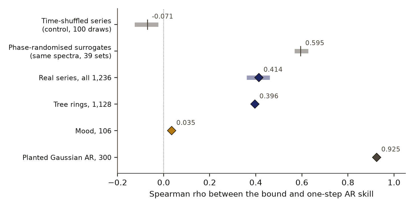
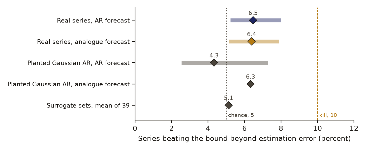
The phase-surrogate control keeps each series' spectrum and makes it Gaussian and stationary. On those sets the bound should rank skill well and the violation rule should fire 5 percent of the time. Over the 39 surrogate sets the pooled rho ran from 0.568 to 0.628 (5th to 95th percentile, mean 0.595), and the mean violation rate of each set against the other 38 was 5.1 percent. The violation rule is calibrated.
Planted linear series: 300 Gaussian autoregressive series of order 1 to 4 with random stable roots and lengths drawn from the real tree and mood lengths, whose true bound is known analytically. The estimated bound correlated 0.925 with skill and 0.946 with the true bound, with a mean bias of -0.020 and a mean absolute error of 0.077. Their violation rate was 4.3 percent (2.5 to 7.3).
Planted nonlinear series: 50 noisy logistic maps of length 400, a deterministic nonlinear system that a linear forecast handles poorly. The analogue forecaster beat the linear bound in all 50, with median skill 0.987 against a median bound of 0.084, while the linear forecast violated in 6 percent. The nonlinear check can see nonlinear predictability when it is there.
Results
All 1,236 series were kept. Figure 2 sets the ranking against both controls and Table 1 gives the main numbers.
One minus spectral flatness ranked held-out one-step forecast skill with Spearman rho 0.414 (95% interval 0.361 to 0.461), against a time-shuffled control whose 95th percentile was -0.023. The ranking passed the Benjamini-Hochberg correction. A separate permutation of the pairing between bound and skill gave p 0.0005.
Spearman rho between bound and skill (higher: closer ranking)
- rho on the real series
- control, 5th to 95th percentile
- control mean
- no ranking
Data behind chart 2 7 rows
| Quantity | Series | Rho | Control 5th pct | Control mean | Control 95th pct | Draws or sets |
|---|---|---|---|---|---|---|
| Real series, all | 1,236 | 0.414 | ||||
| Time-shuffled control | 1,236 | −0.126 | −0.071 | −0.023 | 100 | |
| Phase-surrogate control | 1,236 | 0.568 | 0.595 | 0.628 | 39 | |
| Tree rings | 1,128 | 0.396 | −0.030 | 100 | ||
| Mood | 106 | 0.035 | 0.098 | 100 | ||
| Planted Gaussian series | 300 | 0.925 | ||||
| Later round, test split of the same series | 585 | 0.404 | 0.595 |
Read from result.json (main run), run 20261030T003557Z. SHA-256 of the run's file d7c106b84548d9b9859404325c8529c1aaef21923c5ebe3ffa0b2d1229c66c28 and of the published copy 409175886f0ccba99ed9d57f05b7878dcc68f3ba163f4e9e2c36ed077bbe4aef. In the copy, file paths are cut to the file name and the layout (indentation, line endings) may differ; every value is the same.
Read from round1-result.json (later round on a split of the same series), run 20261030T025631Z. SHA-256 of the run's file 84038a29a80a5b7727fda1635d62afd0abb6e3abc7ad6d0c71b084f17dadae3c and of the published copy 9b8c5eabfbd8b9d78e64d9788bf46173e8407e011fc9ab2dd33c5caf5feee7e2. In the copy, file paths are cut to the file name and the layout (indentation, line endings) may differ; every value is the same.
Real series tracked the bound less tightly than copies with the same spectra: rho 0.414 against 0.568 to 0.628 on 39 phase-randomised surrogate sets. The real value sits below every one of the 39 sets. Gaussian stationary series with the same spectra let the bound rank skill better than the real series do.
80 of 1,236 series (6.5 percent, 5.2 to 8.0) beat the bound beyond estimation error, under the preregistered 10 percent kill. The rate sits above the 5 percent expected by chance (binomial p 0.013, which passed the correction), yet no single series survives a Benjamini-Hochberg correction across series: 0 of 1,236. With 39 surrogates the smallest p value one series can reach is 0.025, far above what that correction needs across 1,236 series, so no series could have passed and this line rules nothing out. Figure 3 shows the rates. Without the surrogate rule the bound would look much weaker as a ceiling: AR skill exceeded the point bound in 36.4 percent of real series and in 45.7 percent of planted Gaussian ones, where the bound is true by construction.
percent of series that beat the bound (lower: the ceiling holds)
- Linear autoregressive forecast
- Nonlinear analogue forecast
- 95% Wilson interval, where the result file gives one
- chance, 5%
- limit, 10%
Data behind chart 3 7 rows
| Series | Forecast | n | Beat the bound (%) | 95% Wilson interval (%) | Skill above the point bound, no surrogate rule (%) |
|---|---|---|---|---|---|
| Real | linear | 1,236 | 6.5 | 5.2 to 8.0 | 36.4 |
| Real | nonlinear analogue | 1,236 | 6.4 | 5.2 to 7.9 | 25.6 |
| Planted Gaussian | linear | 300 | 4.3 | 2.5 to 7.3 | 45.7 |
| Planted Gaussian | nonlinear analogue | 300 | 6.3 | not in the file | |
| Planted nonlinear (logistic maps) | linear | 50 | 6.0 | not in the file | |
| Planted nonlinear (logistic maps) | nonlinear analogue | 50 | 100.0 | not in the file | |
| Phase surrogates, mean over sets | linear | 1,236 | 5.1 | not in the file |
Read from result.json (main run), run 20261030T003557Z. SHA-256 of the run's file d7c106b84548d9b9859404325c8529c1aaef21923c5ebe3ffa0b2d1229c66c28 and of the published copy 409175886f0ccba99ed9d57f05b7878dcc68f3ba163f4e9e2c36ed077bbe4aef. In the copy, file paths are cut to the file name and the layout (indentation, line endings) may differ; every value is the same.
A nonlinear analogue forecaster beat the bound in 6.4 percent of series, the same as its false rate of 6.3 percent on planted Gaussian series, so no predictability beyond the linear bound turned up. Its median skill was 0.044 below the linear model's. The secondary verdict for nonlinear excess failed.
Table 2 breaks the result down by kind of series.
Tree rings carry the pooled result: rho 0.396, p 0.0099, passing the correction, with a median AR order of 2. Mood gives rho 0.035 (p 0.19, failing the correction), because its bound, median 0.024, leaves almost nothing to rank, and its median skill is below zero. Both power series beat the bound. Their load drifts between the two halves, so they are not stationary, and the bound does not apply to them.
Two secondaries ran as planned. The spectral exponent alone, the slope of the log spectrum against log frequency on the training half, ranked skill at rho 0.394 against 0.414 for flatness, so that verdict failed; the two measures correlate at 0.697 and the result file gives no interval on their difference, so we treat them as close. On sensitivities, the Welch estimator with segments of one eighth of the series gave rho 0.399 with a lower median bound of 0.099, a second Welch rule gave 0.441, and linear detrending in place of demeaning gave 0.423.
A later round of our own, run on 30 October 2026 with its own preregistration, tested four drift-aware versions of the bound on a split of the same tree-ring and mood series, choosing on 649 development series and testing on 585. None beat the original, which was chosen. On the 585 test series the original gave rho 0.404 against 0.595 on surrogates. The gap between real and surrogate series repeated on a split of the same data, not on new series.
Discussion
The bound does two things on real series. It ranks them: series with peaked spectra in the first half are the ones a linear model forecasts best in the second half. And, read with its own surrogate envelope, it holds as a ceiling for about 94 percent of series. The cheap number is useful for triage, the use Wang and colleagues [4] propose for their spectral score.
The part worth more work is the gap. Real series rank less well than Gaussian stationary series with identical spectra. Three explanations compete, and this study does not separate them. Fitting a model on half a series adds estimation error, which the surrogates share but may not share in full. Real series drift, as the power logs do in the extreme, and a bound estimated on one half then describes the other half less well. And real series may carry non-Gaussian structure, though the analogue forecaster found none that it could use. The violation rate sitting slightly above 5 percent fits the same picture: a small excess spread thinly across many series and not concentrated in a few series that clearly break the bound.
The surrogate rule matters for anyone who uses such a bound. Compared against the point bound, skill looked like a breach in a third of real series and almost half of planted ones. Compared against each series' own surrogates, breaches fell to the chance rate in planted data and slightly above it in real data.
Limitations
- Tree rings are 91 percent of the series and arrive already standardised, so the pooled rho may come partly from the mix of groups. Mood contributes almost no range of bound to rank.
- The study does not separate estimation error, drift and non-Gaussian structure as causes of the gap between real and surrogate series.
- The bound is a ceiling only after estimation error is allowed for; as a point value it was beaten in 36 percent of real series.
- Only one-step forecasts were tested. Nothing here covers longer horizons.
- The analogue forecaster finding no excess says nothing about stronger nonlinear models.
- The power logs are not public and are not stationary across halves.
- The bound itself is classical, and close heuristics exist; what is tested here is how it behaves on real series against their surrogates.
- The study was not blind to the kinds of data, and scoring was done by our own code.
Evidence
Held. A preregistration with working controls and known answers, on real data, but it tests a 1940s bound on mostly one type of data. The gap between real series and their surrogates is the part worth expanding; a later study of ours repeated it on a split of the same data, and it has not been tested on new series.
Figures
These are the paper's own figures, numbered as in the PDF, and each "Figure" reference in the text points here. The charts on this page redraw the same results from the result files and carry their own numbers.
Tables
| Quantity | Value | Interval or comparison |
|---|---|---|
| Spearman rho, bound against AR skill | 0.414 | 0.361 to 0.461 |
| Time-shuffled control, 95th percentile | -0.023 | p 0.0099, 100 draws |
| Phase-surrogate sets, rho | 0.595 mean | 0.568 to 0.628, 39 sets |
| Violations, AR forecast | 80 of 1,236, 6.5 percent | 5.2 to 8.0 |
| Violations, analogue forecast | 79 of 1,236, 6.4 percent | 5.2 to 7.9 |
| Median bound | 0.203 | |
| Median AR skill | 0.129 | |
| Median excess, skill minus bound | -0.063 | |
| AR skill above the point bound | 36.4 percent | planted AR: 45.7 percent |
| Group | Series | Rho | Shuffle cut | Median bound | Median skill | Violations |
|---|---|---|---|---|---|---|
| Tree rings | 1,128 | 0.396 | -0.030 | 0.213 | 0.146 | 6.1 percent |
| Mood | 106 | 0.035 | 0.098 | 0.024 | -0.072 | 8.5 percent |
| Machine power | 2 | none | none | 0.638 | 0.838 | 2 of 2 |
Appendix A. The preregistered verdicts
Each verdict is a set of rules written before the run. A verdict passes only when every rule holds. Values are read from the run's result file.
| Verdict | Deciding rule | Value | Holds |
|---|---|---|---|
| Planted linear series | rho of estimate with skill at least 0.7; with true bound at least 0.8; violations at most 0.10 | 0.925; 0.946; 0.043 | yes |
| Planted nonlinear series | analogue violations at least 0.5; AR violations at most 0.10 | 1.0; 0.06 | yes |
| Flatness tracks skill | rho above shuffle 95th percentile (-0.023); passes the correction; bootstrap lower bound above 0 | 0.414; yes; 0.361 | yes |
| Bound holds | AR violation rate at most 0.10 | 0.065 | yes |
| Phase surrogates keep the bound | surrogate 5th percentile above shuffle 95th percentile; mean surrogate violation rate at most 0.10 | 0.568; 0.051 | yes |
| Adopt the flatness unit | every rule of the planted linear, tracking and holding verdicts | all hold | yes |
| Nonlinear beats the linear bound, secondary | analogue violations above 0.10; above its planted rate (0.063); passes the correction | 0.064; yes; yes | no |
| Exponent alone, secondary | absolute rho of spectral exponent with skill at least the flatness rho (0.414) | 0.394 | no |
Numbers recorded in our publication register
| What | Value |
|---|---|
| Sample | 1,236 series; 1,128 tree-ring, 106 mood, 2 power |
| Main estimate and interval | rho 0.414 [0.361, 0.461]; violation 6.5% [5.2%, 8.0%] |
| Forecast against outcome | the thresholds set in advance were passed; real series ranking below every surrogate set was not forecast |
| Known-answer check | planted AR rho 0.925 skill, 0.946 true bound, violation 4.3%; logistic map flagged 100% |
As recorded in the publication register, the summary row each finding gets; the paper's own numbers above were re-read from the result files.
What lowers it
- blinding Not blind. A change of estimator before the lock is disclosed in the paper. from our publication register, on blinding
- failed check Controls: the series shuffle, the phase surrogates and the planted autoregressive and logistic-map series all worked; two side forecasts failed, that a nonlinear forecaster beats the linear bound and that the spectral slope alone ranks skill. from our publication register, on controls
- depth of reading The cited literature was read at the level of abstracts, search summaries and publisher pages; full texts were not read. from the Verified section
What holds it up
- scoring Scored by code against rules fixed in advance. from our publication register, on who scored it
- preregistration Preregistered and hash-locked before the run (sha256 fe8ddb06). from the Reproduce section
- replication Rechecked by F91 (flatness bound against drift-aware versions): On 649 development series no drift-aware option beat the original bound (rho 0.350 to 0.398 against 0.414); same data family, not independent. from a later finding
- open data Part of the data is public and part is not; the data licence line under Reproduce says which. from our publication register, on the data licence
Where the claim stands
- lead
- hypothesis
- thesis
- conjecture
- theorem
- law candidate
- killed
A preregistration with pass-or-fail rules is on file, which this rung needs. The next rung needs a named rival reading beaten by a decisive observation, and none is on file. Tier B*: A preregistration with working controls and known answers, on real data, but it tests a 1940s bound on mostly one type of data. The gap between real series and their surrogates is the part worth expanding; a later study of ours repeated it on a split of the same data, and it has not been tested on new series.
Trail
Versions
- v4 2026-11-14, this page corrected, 1 item; the PDF and its BuildTeX source are still paper version 1.0
- v3 2026-11-09, paper version 1.0, first published PDF sha256 03bf9be3b7776174
- v2 2026-10-30, dated correction, 1 item
- v1 2026-10-29, entered in the findings ledger
Corrections
2026-11-14 scope found by a review of the published pages
A review of the published page found one line that reads as a result and could not have come out otherwise. now No single series survived the correction across series, 0 of 1,236; with 39 surrogates per series the smallest possible p value is 0.025, so none could have. The results now say so. The reader section said the bound sorted tree-ring and mood series; for mood the rank correlation was 0.035 and failed its correction, so the sentence now names tree rings only.
2026-10-30 wording found by a later study of ours
A follow-up round tested drift-aware versions of the bound on a split of the same series; none beat the original. now Added to the results here.
2026-10-29 wording found by the study itself, before publication
The first bound estimator underestimated the true bound on synthetic data, and the tapered periodogram became primary. now Disclosed in the preregistration and in the preregistration section here.
Standing, and the ledger entries it rests on
2026-10-30 held F91
Set by hand from findings ledger entry F91, dated 2026-10-30: flatness bound against drift-aware versions. Rests on findings ledger, F91 C2.
Each correction is a dated note; the findings ledger is never rewritten, and a note governs where it differs.
Ledger and version dates up to publication are local dates in US Pacific time. Clock times in the text are UTC, seven or eight hours ahead, so a lock or a run stamped just after midnight UTC belongs to the previous local day. Corrections from 14 November 2026 on are dated in UTC.
References
- Davis, H. T. and Jones, R. H. (1968). Estimation of the innovation variance of a stationary time series. Journal of the American Statistical Association 63 (321), 141-149. doi:10.1080/01621459.1968.11009229 abstract or summary, 2026-11-09: abstracts, search summaries and publisher pages; full text not read used in Introduction and motivation
- Luati, A., Proietti, T. and Reale, M. (2012). The variance profile. Journal of the American Statistical Association 107 (498), 607-621. abstract or summary, 2026-11-09: abstracts, search summaries and publisher pages; full text not read used in Introduction and motivation
- Goerg, G. M. (2013). Forecastable component analysis. Proceedings of the 30th International Conference on Machine Learning, PMLR 28 (2), 64-72. arXiv:1205.4591 abstract or summary, 2026-11-09: abstracts, search summaries and publisher pages; full text not read used in Introduction and motivation
- Wang, R., Klee, S. and Roos, A. (2025). Time series forecastability measures. arXiv:2507.13556 abstract or summary, 2026-11-09: abstracts, search summaries and publisher pages; full text not read used in Introduction and motivation, Discussion
- Theiler, J., Eubank, S., Longtin, A., Galdrikian, B. and Farmer, J. D. (1992). Testing for nonlinearity in time series: the method of surrogate data. Physica D 58, 77-94. doi:10.1016/0167-2789(92)90102-S abstract or summary, 2026-11-09: abstracts, search summaries and publisher pages; full text not read used in Methods
- International Tree-Ring Data Bank. NOAA National Centers for Environmental Information, World Data Service for Paleoclimatology. Standard chronologies, retrieved October 2026. https://www.ncei.noaa.gov/products/paleoclimatology/tree-ring run here Licence: ITRDB, a public archive; the openESM datasets under CC BY 4.0, as the paper's data section states; the two power logs are our own and not public used in Data and provenance
- openESM experience-sampling datasets 0008 Westhoff, 0018 Bailon, 0062 Neubauer and 0076 Bayer. Zenodo, CC BY 4.0. doi:10.5281/zenodo.17347510, doi:10.5281/zenodo.22763396, doi:10.5281/zenodo.17347974, doi:10.5281/zenodo.22911022 run here Licence: ITRDB, a public archive; the openESM datasets under CC BY 4.0, as the paper's data section states; the two power logs are our own and not public used in Data and provenance
- Traxler, R. P. (1889). The Principles of Mechanics as Applied to the Solar System. San Francisco: C. A. Murdock and Co. Internet Archive item principlesofmech00traxiala. read in full: the scan, read in full on the Internet Archive used in Introduction and motivation
Cited by later findings
- F91 held, flatness bound against drift-aware versions, 2026-10-30 (record findings ledger, F91 C2). On 649 development series no drift-aware option beat the original bound (rho 0.350 to 0.398 against 0.414); same data family, not independent.
Reproduce
Data
- International Tree-Ring Data Bank. Licence: ITRDB, a public archive; the openESM datasets under CC BY 4.0, as the paper's data section states; the two power logs are our own and not public. https://www.ncei.noaa.gov/products/paleoclimatology/tree-ring
- openesm. Licence: ITRDB, a public archive; the openESM datasets under CC BY 4.0, as the paper's data section states; the two power logs are our own and not public. https://doi.org/10.5281/zenodo.17347510
Preregistration
sha256 fe8ddb061ffc02c3f22d89222fb6b5e20baf402e128c930a85242f161207dae7
plan 4b0268f175706e5803a21cd91d320ebb96e62f3fe97a67639030c3a7bd2c3d26
Steps
- Data: ITRDB standard chronologies for the conterminous United States of at least 200 years with no gaps; the four openESM mood datasets named above, series of at least 100 prompts in prompt order. The two power logs are not public.
- Split each series in half by time. On the training half, demeaned, compute the Hann-tapered periodogram and eq. 2, then the bound of eq. 3.
- Fit an AR model by least squares with order chosen by AIC up to the smaller of 20 and one tenth of the training length; score eq. 4 on the test half from the true past.
- Build 39 phase-randomised surrogates of each whole series, run the same pipeline, and flag violations by eq. 5 at 38 of 39.
- Correlate bound and skill across series with Spearman rho; run 100 time-shuffled controls and a 1,000-resample bootstrap.
- Preregistration SHA-256: fe8ddb061ffc02c3f22d89222fb6b5e20baf402e128c930a85242f161207dae7. Plan SHA-256: 4b0268f175706e5803a21cd91d320ebb96e62f3fe97a67639030c3a7bd2c3d26. Run 20261030T003557Z. Result file SHA-256: d7c106b84548d9b9859404325c8529c1aaef21923c5ebe3ffa0b2d1229c66c28.
Cost. The analysis took 272 seconds on one desktop computer. Machine energy over the run window was 47.1 kJ, shared with other work on the same machine. The study was not re-run for this paper.
Downloads
- Whitepaper, PDF F76.pdf, 3.3 MB
- BuildTeX source F76.bld, 38 KB
- Build receipt F76.buildtex.json, 1 KB
- BuildLang doc module doc.bld, 5 KB, imported by the source
The PDF is typeset by BuildTeX from F76.bld, which is written from the same source as this page. The receipt records the source's SHA-256 and the PDF's (03bf9be3b777), so anyone can rebuild it and compare. The copy here has its hidden author field blanked, as the site does for every file it publishes; blank the same field in a rebuild before comparing. The name stays on the first page.
Verified
Verified on 2026-11-09. On 9 November 2026 the series counts by group, the pooled and group rho values with their intervals and shuffle cuts, the violation counts, rates and Wilson intervals, the binomial p values, the medians, the share above the point bound, every control percentile and mean, the planted linear and nonlinear values, the secondaries and sensitivities, and all eight verdicts were re-read from the run's result file; they match the findings ledger. The preregistration's SHA-256 and the result file's SHA-256 match the hashes recorded beside them. The follow-up values (649 and 585 series, rho 0.404 and 0.595, the original bound chosen) were re-read from the later round's result file. Both data figures were drawn by a script that reads only the result file.
Not checked. The study was not re-run for this paper. The literature in the introduction was found by searches run on 9 November 2026 and read at the level of abstracts, search summaries and publisher pages; the full texts of the cited papers were not read.
Terms on this page
Each term is defined where it is first used on this page. Each name below opens its entry in the findings glossary, which lists every page that uses it.
- power spectrum time-series analysis and signal processing first use
- spectral flatness signal processing (speech coding) and the theory of stationary processes first use
- weakly stationary probability and time-series analysis first use
- Kolmogorov-Szego bound the theory of weakly stationary processes first use
- preregistration research method (metascience) first use
- kill condition research method (our usage, after Popper's falsification) first use
- verdict research method (our usage) first use
- tapered periodogram spectral estimation first use
- autoregressive model time-series statistics first use
- AIC statistical model selection first use
- one-step skill forecast verification first use
- Spearman rho statistics (rank correlation) first use
- phase-randomised surrogate nonlinear time-series analysis (surrogate data) first use
- violation of the bound our usage in this study first use
- Wilson interval statistics (binomial proportions) first use
- analogue forecaster nonlinear time-series prediction (method of analogues) first use
- Benjamini-Hochberg correction statistics (multiple testing) first use
- control statistics and experimental design first use
- planted check research method; called a positive control in experimental science first use
- p value (from draws) statistics first use
To report an error, name the finding, the claim number and the source on the Work page, which gives the address. Accepted corrections join the Trail with their date.