
Findings F38 Psychology and perception, Method and statistics found 2026-10-29
Forecasts drift, mood steps or drifts in many people; simulated five-a-day prompts miss fast emotion
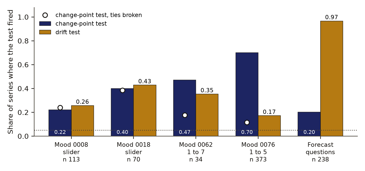
Crowd forecasts drift toward the answer in 97 percent of 238 questions, as expected. On slider mood scales a change-point test fired in 22 and 40 percent of people and a drift test in 26 and 43 percent, against about 5 percent for a stationary series. Eleven of 20 preregistered predictions did not hold, the switching test could not fire, and the sampling result comes from simulation.
- Tier
- B, signal
- Outcome
- mixed
- Rung
- hypothesis
- Corrections
- 4, latest 2026-11-14
- Version
- v3, 2026-11-14
- Redo it
- Reproduce
Download PDF 567 KB BuildTeX source F38.bld
What this means for a reader
A crowd forecast moves steadily toward the right answer as the question nears its end, so its average over the whole period describes no moment of it. Mood reported on a phone is steadier, but in a large minority of people it steps or drifts over the weeks of a study by more than their own hour-to-hour carryover explains. A study that prompts five times a day also cannot see feelings that rise and fade within the hour: they show up as noise. More than half of what we predicted about these data was wrong, and one of our tests was built so that it could not give a positive answer, which we report as a defect.
Objection
Eleven of 20 predictions did not hold, and one that held could not have failed. A further one, that the inventory series are too short to test, is a statement about series length.
What would change the call. Rerun with surrogates that keep each series' own distribution of values and a tie-aware change-point cost on an independent experience-sampling dataset, plus a continuous physiological signal for tests under one hour.
From the paper's first stated limitation; our register records no separate objection.
Abstract
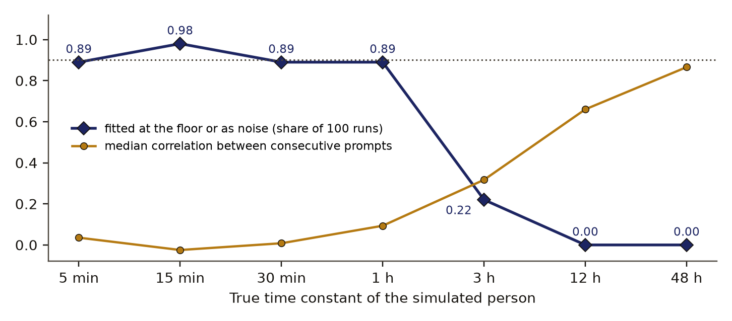
Most statistics for a series of measurements assume the process behind it holds still. We built tests for three ways it can move (a step, a slow drift, a switch between two states), checked each on synthetic series with known answers, and ran them on crowd forecasts and on mood reported several times a day. Twenty predictions were fixed in advance. The ledger scores 9 of the 20 as held and 11 as not held, and one of the 9 held only because its rule could never fire. In 238 forecast questions the drift test fired on 97 percent and 96 percent ended nearer the answer than they began, by a median 0.24 in probability, which is what a crowd converging on an outcome is expected to do. On the two slider datasets the change-point test fired in 22 and 40 percent of people and the drift test in 26 and 43 percent, against about 5 percent per test for a stationary AR(1) series. On the 1 to 7 and 1 to 5 scales the raw change-point rates of 47 and 70 percent fell to 18 and 12 percent once ties were broken, so most of those detections came from the rating scale. The switching test used 19 surrogates, so its smallest p value was 0.05 and the rule "p below 0.05" could never fire; no claim about switching is made. Simulated people whose mood relaxes in 5, 15 or 30 minutes, sampled five times a day for 20 days with no measurement noise, were fitted at the sampling floor or with a noise share of 0.8 or more in 89, 98 and 89 percent of 100 runs, against a preregistered bar of 90 percent.
c1 observed, evidence for claim 1
- The numbers in claim 1
- 9; 20; 11 matches the result file, 2026-11-14
- Basis
- observed: measured in this study, with a result file
c2 observed, evidence for claim 2
- The numbers in claim 2
- 238; 97; 96; 0.24 matches the result file, 2026-11-14
- Basis
- observed: measured in this study, with a result file
c3 observed, evidence for claim 3
- The numbers in claim 3
- 22; 40; 26; 43; 5; 1 matches the result file, 2026-11-14
- Basis
- observed: measured in this study, with a result file
c4 observed, evidence for claim 4
- The numbers in claim 4
- 1; 7; 5; 47; 70; 18; 12 matches the result file, 2026-11-14
- Basis
- observed: measured in this study, with a result file
c5 observed, evidence for claim 5
- The numbers in claim 5
- 19; 0.05 matches the result file, 2026-11-14
- Basis
- observed: measured in this study, with a result file
c6 observed, evidence for claim 6
- The numbers in claim 6
- 5; 15; 30; 20; 0.8; 89; 98; 100; 90 matches the result file, 2026-11-14
- Chart 1
- How the sampling floor was sized by simulation.
- Chart 2
- Simulated people fitted at the sampling floor or as noise, by how fast their mood really changes.
- Basis
- observed: measured in this study, with a result file
Introduction
A series is stationaryDefinition: stationary probability and time-series analysis A series whose mean and autocovariance do not change over time. Excludes series with trends, level shifts or drifting variance. full definition when its mean and its autocovariance do not change over time, a term from time-series analysis that excludes trends, level shifts and drifting variance. Measures such as an autocorrelation or a spectrum summarise a whole record in a few numbers, and those numbers describe the process only if it is stationary. A recent primer on non-stationarity in psychological time series [4] warns, in the summary we read, that ignoring a trend biases estimates and distorts their sampling distributions.
Mood research meets the problem in experience samplingDefinition: experience sampling psychology (methods) A study design in which people answer short questions on a phone several times a day, so that mood is recorded close to the moment it is felt. Excludes one-off questionnaires and recall of past weeks. full definition, a design in which people answer short questions on a phone several times a day. Such data are sparse and unevenly spaced, and how spacing biases models fitted to them is a studied question [7]. A simulation study found that popular time-series tools lose the dynamics of a toy emotion model once measurements are as sparse as experience sampling, and its authors suspected a mismatch between prompts hours apart and processes that unfold over seconds to minutes [5]. A Monte Carlo study of continuous-time autoregressive models found estimates degraded when the process was observed more slowly than it ran [6].
We asked three things. Which of the processes we hold data on are stationary, by tests that can tell a step from a drift? How widely do people differ in the time their mood takes to relax? And what is the fastest mood process a five-a-day schedule can measure? The decision this informed was which of our own stationary measures may be applied to which data. Our searches returned the work above and no published share of experience-sampling participants whose series fail a stationarity test; that is what two searches returned and no proof that none exists.
Preregistration and design
The preregistrationDefinition: preregistration research method (metascience) A dated written plan for a study, fixed and hash-locked before any result is seen: the question, the data, the statistic, the controls, the forecasts and the kill conditions. Excludes a plan revised after looking at the outcome, and a protocol written only for the record after the run. full definition, a dated plan fixed and hashed before any result is seen, was written on 29 October 2026 and its SHA-256 recorded at 15:54:42 UTC that day, before any measure was run on any real series. Before writing it we had seen file headers, counts of people and prompts, record spans, and the results of the synthetic recovery runs. It fixes 20 predictions, each scored held or not held as written by our own code and reading of the result files, with nothing re-scored after the run and every unplanned analysis labelled exploratory. Each scored prediction is a verdictDefinition: verdict research method (our usage) The pass or fail of one preregistered rule set against the run's numbers, read off by code. Excludes an interpretation written after reading the numbers. full definition. Appendix A lists all 20.
Data and provenance
- Good Judgment Project survey forecasts, years 1 to 4, CC0 1.0 [1]. We kept closed binary questions open for at least 60 days with forecasts on at least 60 days: 238 questions. Each series is the daily median probability given to the outcome that occurred, with empty days carried forward.
- Four datasets from the openESM database [2], each CC BY 4.0: 0008 (valence on a 0 to 100 slider), 0018 (valence on a slider from -50 to 50), 0062 (happiness, 1 to 7) and 0076 (positive affect, 1 to 5). People with at least 60 usable prompts and 3 distinct values were kept: 113, 70, 34 and 373, in total 590. Only distributions across people are reported.
- Forest Inventory and Analysis remeasurements for Oregon and Washington [3], a United States Government work in the public domain: annual mortality share and survivor growth by remeasurement year, 14 and 12 years.
- Two looping animations rendered by our own software, 288 and 144 frames, tiled four times. They are a known periodic control and are not public data.
Methods
The three tests
Each test compares a series with surrogatesDefinition: surrogate series time-series statistics A simulated series that keeps chosen properties of a real one, here its length, mean, standard deviation and lag-1 memory, and nothing else, so a statistic on the real series can be compared with what those properties alone produce. Excludes the real series' distribution of values, which a Gaussian surrogate does not copy. full definition of itself: simulated series from an AR(1) processDefinition: AR(1) process time-series statistics A series in which each value is the mean plus a fixed fraction of the previous value's distance from the mean, plus fresh random noise. Excludes steps, drifting coefficients, switching between states and long memory. full definition fitted to it, in which each value is the mean plus a fraction of the previous value's distance from the mean plus Gaussian noise ,
with the same length, mean, standard deviation and as the real series. A surrogate keeps the memory between neighbouring values and has no step, drift or switching. For a statistic that is times matched or beaten among surrogates,
so the smallest possible value is .
- Change-pointDefinition: change point time-series statistics A time at which the mean or variance of a series changes. Here found by a penalised search that adds a change only when it improves the fit by more than a fixed penalty. Excludes gradual change, which the drift test reads. full definition test: the number of changes in mean or variance found by a penalised search (PELT, penalty , segments of 5 or more), against 99 surrogates.
- Drift testDefinition: drift test time-series statistics, our usage A comparison of an autoregressive model whose coefficient follows a random walk with one whose coefficient is fixed, by likelihood ratio. Excludes a drift of the mean level alone with a constant coefficient, which this test does not target. full definition: a model whose AR coefficient follows a random walk, , fitted by a Kalman filter; the likelihood ratio against a fixed coefficient, against 49 surrogates.
- Switching testDefinition: switching test econometrics (Markov-switching models) A comparison of a model with two hidden states, each with its own level and spread, that the series moves between, with a single AR(1), by likelihood ratio. Excludes a one-way step, which the change-point test reads. full definition: a two-state Markov-switching AR(1) against a single AR(1), likelihood ratio, against 19 surrogates.
A series is labelled switching if the third test gives p below 0.05 with at least 3 switches, else shift if the first does, else drift if the second does, else stationary. In a stationary AR(1) world each test fires about 5 percent of the time.
Timescales
For each person we fitted an Ornstein-Uhlenbeck time constantDefinition: Ornstein-Uhlenbeck time constant stochastic processes The time over which a quantity that relaxes toward its mean loses about 63 percent of a deviation, fitted here from each person's prompts at their real times with a separate noise term. Excludes a second, slower or faster timescale in the same person, which this fit does not model. full definition to the real prompt times. The model is a mood that relaxes toward its mean, observed with independent noise, so two prompts hours apart correlate as
where is the share of variance that is noise. A person is at the sampling floorDefinition: sampling floor our usage, from sampling theory The condition in which a person's fitted time constant is shorter than their median gap between prompts within a day, so the value is not measured. Excludes a claim that the person's mood is fast; noise gives the same reading. full definition when the fitted is shorter than their median gap between prompts within a day; there the time constant is not measured.
The aliasing simulation
AliasingDefinition: aliasing signal processing The misreading that results when a process changes faster than it is sampled, so that the fast change appears in the record as something else, here as noise. Excludes measurement error in the instrument, which is present even with dense sampling. full definition, a term from signal processing, is what happens when a process changes faster than it is sampled: the fast change is recorded as something else, here as noise. We simulated people from eq. 3 with and true from 5 minutes to 48 hours, on a schedule of 20 days with 5 prompts a day, 100 runs per value, and fitted them as real people were fitted.
Controls and planted checks
Every measure first had to recover known values from synthetic series, which is a planted checkDefinition: planted check research method; called a positive control in experimental science Data built so that the right answer is known, run through the same analysis before the real data, to show that the analysis can see the effect when it is there. Excludes any check made on the real data, which cannot show what the analysis misses. full definition: data built so the right answer is known. Over 40 seeds, the median error had to be below the 5th percentile of a shuffled pairing of recovered and planted values and at most half its median. In the recovery file 15 measures pass every rule. Three are recorded as failing and were not used for claims: a spectral slope on five-a-day sampling (ratio 1.04), variance shares in three bands on records under 90 days, and a fit of two timescales in one person (ratios 0.63 and 0.89).
- planted checkPlanted: a known time constantEach simulated mood relaxes toward its mean with a time constant set by us, from 5 minutes to 48 hours.
- measurementThe same fit as on real peopleA time constant and a noise share are fitted to the five-a-day prompts. A fit is at the floor when the time constant is shorter than the gap between prompts.
- rule set in advanceRule: 90 percent at the floor or as noiseFor true time constants of 5, 15 and 30 minutes, at least 90 percent of runs had to be fitted at the floor or with a noise share of 0.8 or more.
- missed the bar89, 98 and 89 percentTwo of the three values fell one run short. At a true time constant of 3 hours the share is 22 percent, and at 12 and 48 hours it is 0.
Read from ns_mood_time.json (timescales and the sampling simulation). SHA-256 of the run's file 0bf1b5011f1592df582403c06eda927b187d69da09da10a0fa0d884e7132bdca and of the published copy 0f243e16ba0c81d212be3dc70c95ec57900cb8170529f2bf4e0ee718d88ea017. In the copy, file paths are cut to the file name and the layout (indentation, line endings) may differ; every value is the same.
Two controlsDefinition: control statistics and experimental design A version of the data with the structure under test removed (for example shuffled or pooled), scored the same way as the real data, so the real score has something to beat. Excludes a comparison with a different dataset or with a published number. full definition, estimators that should fail, passed at first. A single spectral peak passed the test for a frequency sweep (ratio 0.44) and a single AR coefficient passed the test for a drifting one (0.49), because each correlates with the endpoints. The rule was changed so that every moving case is also scored on the movement itself, where both fail at ratio 1.00. A third control showed that a switching model fitted to a shuffled series still recovers the gap between its two levels from the histogram alone; only the durations of the states need time order.
The change-point search was also run on pure noise, 200 series per setting. It reported a change in 2 to 6 percent of white-noise series, and in 83 to 100 percent of AR(1) series with of 0.6 or more. That is why no real series is read from its raw change count and each is judged against AR(1) surrogates.
Results
The ledger scores 9 of the 20 as held and 11 as not held, and one of the 9 held only because its rule could never fire.
The defect
The switching test used 19 surrogates, so its smallest p value was 0.05 and the rule "p below 0.05" could never fire; no claim about switching is made. The switching share is 0 in every dataset by construction, and the prediction that it would be under 15 percent held for that reason alone. An exploratory rerun with "p at most 0.05" and at least 3 switches flagged 47 to 67 percent of people in the mood datasets and 54 percent of forecast questions. Those rates cannot be read as switching: Gaussian surrogates do not copy a bounded, skewed rating scale, and the control above shows the model reads level gaps from the histogram. A surrogate that keeps each series' own distribution of values is the test this needs, and it was not run.
Forecasts
In 238 forecast questions the drift test fired on 97 percent and 96 percent ended nearer the answer than they began, by a median 0.24 in probability, which is what a crowd converging on an outcome is expected to do. Only 1.7 percent of questions were labelled stationary. We had predicted that steps would be the most common label, on the idea that news arrives as jumps; drift was, at 78 percent of questions against 20 percent for shift. The median question ran 126.5 days.
Mood
Table 1 and Figure 1 give the labels and test rates. On the two slider datasets the change-point test fired in 22 and 40 percent of people and the drift test in 26 and 43 percent, against about 5 percent per test for a stationary AR(1) series. These shares rest on 113 and 70 people and have no intervals. We had predicted that more than half the people in every dataset would be labelled stationary, and that held in one dataset of four.
On the 1 to 7 and 1 to 5 scales the raw change-point rates of 47 and 70 percent fell to 18 and 12 percent once ties were broken, so most of those detections came from the rating scale. A coarse scale gives runs of identical answers (a median 45 and 46 percent of consecutive prompts tie in these two datasets), a run of identical values has zero variance, and a Gaussian surrogate never produces one. DequantisingDefinition: dequantising signal processing Adding uniform random noise one scale step wide to values recorded on a coarse scale, so that identical neighbouring answers stop being exactly equal. Excludes any recovery of the finer value the person would have given on a continuous scale. full definition, adding uniform noise one scale step wide, removes the ties; it was an exploratory correction made after the run. On the sliders, where 3 to 4 percent of consecutive prompts tie, the rates barely moved (0.22 to 0.24 and 0.40 to 0.39).
Timescales and the sampling floor
Table 2 gives the fitted time constants. The median lies between 2 and 48 hours in each dataset, and across all 590 people the 5th to 95th percentile range runs from 0.54 to 109 hours, a factor of about 200. Between 13 and 40 percent of people sit at the sampling floor. We had predicted at least 20 percent in every dataset, which held in two.
Simulated people whose mood relaxes in 5, 15 or 30 minutes, sampled five times a day for 20 days with no measurement noise, were fitted at the sampling floor or with a noise share of 0.8 or more in 89, 98 and 89 percent of 100 runs, against a preregistered bar of 90 percent. The prediction missed its bar by one run in a hundred at two of the three values. Its second rule held: the median correlation between consecutive prompts was 0.04, -0.02 and 0.01. Figure 2 shows the whole sweep. A true time constant of 1 hour gave the same 89 percent; at 3 hours the share fell to 22 percent, and at 12 and 48 hours to zero, with fitted values of 11.5 and 37.6 hours. The schedule measures time constants of about 3 hours and longer and folds everything faster into one floor. Sampling theory predicts this; the simulation sizes it for this schedule.
Three further timescale predictions did not hold. A model with two timescales beat one on each person's held-out prompts for 50 to 60 percent of people, where we had predicted at most half; people simulated with one timescale on the same prompt times picked two 46 to 51 percent of the time, so the comparison is close to a coin flip and supports no claim either way. In the 37 people with records of 60 days or more, the median share of variance arriving within a day was 0.72 (interquartile range 0.64 to 0.84) against a predicted range of 0.3 to 0.7, a narrow miss. A two-component mixture was preferred over one on that share (BIC -20.3 against -14.8), against our prediction of a continuum; a cluster of people at the floor beside a spread above it would give the same preference, and that was not tested. As predicted, 27 percent of those 37 people could not be told from their own shuffled series.
The other series
The two animation loops met two of their four predictions: every change point repeated at the same frame in the next loop, and every feature found repeated with the loop. A mode-finding method missed one loop's period because its window of 80 frames was shorter than the 288-frame loop. The forest inventory series, 14 and 12 annual values, are too short for any of the tests; a first run labelled them drifting through a software fault on short series, which was fixed and the faulty output kept. Oregon's mortality share was 0.077 to 0.096 from 2011 to 2020 and 0.125, 0.143, 0.153 and 0.178 from 2021 to 2024. Each year measures a different panel of plots, so this is a description and no test.
Discussion
The forecast result is the cleanest and the least surprising. A crowd's probability for the outcome that happens rises over a question's life, slowly more often than in jumps. Any stationary summary of a forecast series, such as one autocorrelation for the whole question, averages over a process that is changing throughout.
For mood the supported statement is narrower than our write-up first made it. On continuous sliders, a quarter to two fifths of people show a level change or a drifting coefficient beyond an AR(1) with Gaussian noise, each test taken alone. A rejection means "more than AR(1) with a Gaussian marginal", which a long-memory or skewed process also produces. On coarse rating scales the change-point test mostly detected the scale. A researcher fitting one autoregressive model per person to several weeks of slider data should expect it to be wrong in form for a sizeable minority, and should not use a variance-based change-point cost on a 5-point scale.
The sampling result agrees with the simulation literature cited above [5, 6]: a schedule of prompts hours apart cannot recover a process that runs in minutes. Our addition is the size for one common design. With five prompts a day, a person whose feelings turn over within the hour is indistinguishable from a person who is half noise. Measuring that person needs a continuous signal.
The defect has a general form. A surrogate count sets the smallest p value a test can return, and a threshold at or below that value makes the test silent. The count has to be chosen from the threshold.
Limitations
- Eleven of 20 predictions did not hold, and one that held could not have failed. A further one, that the inventory series are too short to test, is a statement about series length.
- The switching test could not fire. No switching result exists, in either direction.
- The headline shares have no intervals. They rest on 113, 70, 34 and 373 people and 238 questions.
- The surrogates copy mean, variance and lag-1 memory only, with Gaussian noise. Bounded probabilities and rating scales sit outside that family.
- The tie correction and the switching rerun were exploratory and made after the results were seen.
- The stationarity tests order prompts and ignore the gaps between them, including nights.
- The aliasing result comes from simulation of one model and one schedule, and follows from sampling theory. It missed its own bar of 90 percent at two of three values.
- That forecasts move toward the answer is expected, and the series was defined as the probability of the realised outcome.
- Forest inventory years are different plot panels; those numbers are descriptive.
- Scoring was done by our own code and our own reading of the result files, and was not blind.
Evidence
Mixed. Eleven of 20 predictions did not hold. The switching test used 19 surrogates, so its smallest p was 0.05 and its rule could not fire: no switching result exists. The aliasing prediction missed its 90 percent bar at two of three values (89, 98, 89 percent of 100 runs). The within-day variance share was 0.72 against an upper bound of 0.7. On 1 to 5 and 1 to 7 scales the change-point rates of 70 and 47 percent fell to 12 and 18 percent once ties were broken.
Figures
These are the paper's own figures, numbered as in the PDF, and each "Figure" reference in the text points here. The charts on this page redraw the same results from the result files and carry their own numbers.
Tables
| Series | n | Stationary | Shift | Drift | Change-point test | Drift test |
|---|---|---|---|---|---|---|
| Mood 0008, slider | 113 | 0.58 | 0.22 | 0.19 | 0.22 | 0.26 |
| Mood 0018, slider | 70 | 0.36 | 0.40 | 0.24 | 0.40 | 0.43 |
| Mood 0062, 1 to 7 | 34 | 0.32 | 0.47 | 0.21 | 0.47 | 0.35 |
| Mood 0076, 1 to 5 | 373 | 0.25 | 0.70 | 0.05 | 0.70 | 0.17 |
| Forecast questions | 238 | 0.02 | 0.20 | 0.78 | 0.20 | 0.97 |
| Dataset | n | Median | 5th to 95th percentile | At floor | Gap |
|---|---|---|---|---|---|
| 0008 | 113 | 10.0 | 1.6 to 72 | 0.23 | 3.2 |
| 0018 | 70 | 17.0 | 1.8 to 809 | 0.13 | 3.4 |
| 0062 | 34 | 13.5 | 1.2 to 346 | 0.18 | 2.0 |
| 0076 | 373 | 3.5 | 0.29 to 49 | 0.40 | 2.7 |
| All | 590 | 5.9 | 0.54 to 109 | none | none |
Appendix A. The preregistered verdicts
Each prediction is scored as written. Values are read from the study's result files.
| Prediction | Value | Outcome |
|---|---|---|
| Mood: stationary label over half in every dataset | 0.58, 0.36, 0.32, 0.25 | not held |
| Mood: shift or drift above 14 percent in two datasets and under 40 in all | 0.42, 0.64, 0.68, 0.75 | not held |
| Mood: switching under 15 percent | 0, by the defect | held, could not fail |
| Forecasts: at least 60 percent not stationary | 0.98 | held |
| Forecasts: shift the most common label | shift 0.20, drift 0.78 | not held |
| Forecasts: at least 75 percent rise toward the answer | 0.96 | held |
| Loops: top mode at a multiple of the loop frequency within 1 percent | one loop 0.5 percent off; the other 5.3 percent off | not held |
| Loops: change points repeat at the same phase | 22 of 22 in one loop; none found in the other | held |
| Loops: drift path repeats, r above 0.8 | 1.00 and -0.35 (a flat path) | not held |
| Loops: every reported feature repeats with the loop | all repeat | held |
| Median time constant 2 to 48 h; pooled spread at least 1.5 decades | 3.5 to 17.0 h; 2.3 decades | held |
| At least 20 percent at the floor in each dataset | 0.23, 0.13, 0.18, 0.40 | not held |
| Aliasing: at least 90 percent at floor or noise; lag-1 under 0.1 | 0.89, 0.98, 0.89; 0.04, -0.02, 0.01 | not held |
| Two timescales win for at most half; gain under 0.02 nats | 0.55, 0.60, 0.50, 0.56; gains under 0.001 | not held |
| Within-day variance share between 0.3 and 0.7 | 0.72 | not held |
| One mixture component preferred | two preferred | not held |
| At least 20 percent of long records match their shuffle | 0.27 | held |
| Inventory series too short to test | 14 and 12 years | held, by series length |
| Tree growth slower in the second period in both states | -0.01 and 0.00 inches a year | not held |
| Mortality share highest from 2021 on in one state | 2024 and 2022 | held |
Numbers recorded in our publication register
| What | Value |
|---|---|
| Sample | 238 forecast questions; 590 people in four experience-sampling datasets; 37 people with records of 60 days or more |
| Main estimate and interval | no interval on the headline shares; fitted time constants run from 0.54 to 109 hours (5th to 95th percentile) |
| Forecast against outcome | Eleven of 20 predictions did not hold. Two missed narrowly: the aliasing share reached 89 percent against a bar of 90, and the within-day variance share was 0.72 against an upper bound of 0.7 |
| Known-answer check | 15 measures pass recovery on planted cases; a spectral slope on five-a-day sampling and a two-timescale fit fail and were not used |
As recorded in the publication register, the summary row each finding gets; the paper's own numbers above were re-read from the result files.
What lowers it
- blinding Not blind. Labels came from code; the shape of the data had been seen before the lock. from our publication register, on blinding
- failed check Controls: mixed: shuffled and AR(1) surrogates worked; two endpoint-only rules passed estimators that should fail and were tightened; 19 surrogates made the smallest p value 0.05, a defect. from our publication register, on controls
- novelty Nearby work exists; novelty is not shown. from our publication register, on the literature
- depth of reading The cited literature was read at the level of search snippets; full texts were not read. from the Verified section
What holds it up
- scoring Scored by code against rules fixed in advance. from our publication register, on who scored it
- preregistration Preregistered and hash-locked before the run (sha256 cf81972b). from the Reproduce section
- open data Public data. from our publication register, on the data licence
Where the claim stands
- lead
- hypothesis
- thesis
- conjecture
- theorem
- law candidate
- killed
A preregistration with pass-or-fail rules is on file, which this rung needs. The next rung needs a named rival reading beaten by a decisive observation, and none is on file. Tier B: Real data and surrogate controls, but 11 of 20 preregistered predictions did not hold, the switching rule could not fire, and the aliasing part follows from sampling theory.
Trail
Versions
- v3 2026-11-14, paper version 1.0, first published PDF sha256 a224f12983bddafa
- v2 2026-10-31, dated correction, 1 item
- v1 2026-10-29, entered in the findings ledger
Corrections
2026-11-14 scope found by the publication pass
Narrowed the mood statement. now The ledger says a quarter to two fifths of people on sliders step or drift; the files give that range for each test taken alone (0.22 and 0.40; 0.26 and 0.43), and 42 and 64 percent of people carry either label.
2026-11-14 wording found by the publication pass
The ledger counts 16 measures passing recovery. now The recovery file marks 15 as passing every rule, and this paper uses 15.
2026-10-31 number found by a review of our findings ledger
A review of our ledger found that the 97 percent quoted for forecast drift is the rate of the drift test and that the drift label covers 78 percent of questions. now This paper gives both.
2026-10-29 scope found by the study itself, before publication
Found during the run. now The switching test's 19 surrogates made its rule unable to fire; a fault on series shorter than the drift model's burn-in labelled four inventory series as drifting and was fixed; two controls passed an endpoint-only rule and the rule was tightened.
Each correction is a dated note; the findings ledger is never rewritten, and a note governs where it differs.
Ledger and version dates up to publication are local dates in US Pacific time. Clock times in the text are UTC, seven or eight hours ahead, so a lock or a run stamped just after midnight UTC belongs to the previous local day. Corrections from 14 November 2026 on are dated in UTC.
References
- Mellers, B. and others. Good Judgment Project data: survey forecasts, years 1 to 4, and question file. Harvard Dataverse, CC0 1.0. doi:10.7910/DVN/BPCDH5 run here Licence: Good Judgment Project CC0; openESM datasets CC BY 4.0; Forest Inventory and Analysis public domain used in Data and provenance
- Siepe, B. S., Haslbeck, J. M. B., Kloft, M., Büchner, A., Zhang, Y., Fried, E. I. and Heck, D. W. (2026). Introducing openESM: a database of openly available experience sampling datasets. Behavior Research Methods 58, 240. doi:10.3758/s13428-026-03112-y. Datasets 0008, 0018, 0062 and 0076, CC BY 4.0. run here Licence: Good Judgment Project CC0; openESM datasets CC BY 4.0; Forest Inventory and Analysis public domain used in Data and provenance
- USDA Forest Service. Forest Inventory and Analysis DataMart, Oregon and Washington tables. Public domain. https://apps.fs.usda.gov/fia/datamart/CSV/ run here Licence: Good Judgment Project CC0; openESM datasets CC BY 4.0; Forest Inventory and Analysis public domain used in Data and provenance
- Ryan, O. and others. Non-stationarity in time-series analysis: modeling stochastic and deterministic trends. Multivariate Behavioral Research. doi:10.1080/00273171.2024.2436413 abstract or summary, 2026-11-14: search snippets; full text not read used in Introduction
- Recovering within-person dynamics from psychological time series (2021). Multivariate Behavioral Research. doi:10.1080/00273171.2021.1896353. The search result did not show the authors. abstract or summary, 2026-11-14: search snippets; full text not read used in Introduction, Discussion
- Consequences of sampling frequency on the estimated dynamics of AR processes using continuous-time models. PubMed record 37428727. The search result did not show the authors. abstract or summary, 2026-11-14: search snippets; full text not read used in Introduction, Discussion
- De Haan-Rietdijk, S. and others (2017). Discrete- vs. continuous-time modeling of unequally spaced experience sampling method data. PubMed Central record PMC5655034. abstract or summary, 2026-11-14: search snippets; full text not read used in Introduction
Cited by later findings
- No later record in the findings ledger treats this finding.
Reproduce
Data
- Mellers, B. Licence: Good Judgment Project CC0; openESM datasets CC BY 4.0; Forest Inventory and Analysis public domain. https://doi.org/10.7910/DVN/BPCDH5
- Siepe 2026. Licence: Good Judgment Project CC0; openESM datasets CC BY 4.0; Forest Inventory and Analysis public domain. https://doi.org/10.3758/s13428-026-03112-y
- USDA Forest Service. Licence: Good Judgment Project CC0; openESM datasets CC BY 4.0; Forest Inventory and Analysis public domain. https://apps.fs.usda.gov/fia/datamart/CSV/
Preregistration
sha256 cf81972b4975844362218d58ca863efe286f70748879a3064f8b33bb647e8190
plan not recorded
Steps
- Data: Good Judgment Project survey forecasts, Harvard Dataverse, CC0 1.0, doi:10.7910/DVN/BPCDH5; openESM datasets 0008, 0018, 0062 and 0076, CC BY 4.0, doi:10.3758/s13428-026-03112-y for the database; USDA Forest Service FIA DataMart, public domain, https://apps.fs.usda.gov/fia/datamart/CSV/.
- Build each forecast series as the daily median probability of the realised outcome. Keep mood series of 60 or more prompts with 3 or more distinct values.
- For each series fit eq. 1, draw surrogates, and compute eq. 2 for the change-point count (99 surrogates), the drift likelihood ratio (49) and the switching likelihood ratio (19; use 39 or more to make the 0.05 rule able to fire).
- Fit eq. 3 to each person's real prompt times. Simulate eq. 3 on 20 days of 5 prompts for the aliasing sweep.
- Preregistration SHA-256: cf81972b4975844362218d58ca863efe286f70748879a3064f8b33bb647e8190. The study was run by its own scripts, so the files record no plan hash and no run identifier.
Cost. Not recorded The study was not re-run for this paper.
Downloads
- Whitepaper, PDF F38.pdf, 567 KB
- BuildTeX source F38.bld, 37 KB
- Build receipt F38.buildtex.json, 1 KB
- BuildLang doc module doc.bld, 5 KB, imported by the source
The PDF is typeset by BuildTeX from F38.bld, which is written from the same source as this page. The receipt records the source's SHA-256 and the PDF's (a224f12983bd), so anyone can rebuild it and compare. The copy here has its hidden author field blanked, as the site does for every file it publishes; blank the same field in a rebuild before comparing. The name stays on the first page.
Verified
Verified on 2026-11-14. On 14 November 2026 the label shares, test rates, forecast rise share and median, tie shares and dequantised rates, exploratory switching rates, time-constant percentiles, floor shares, held-out comparison shares, within-day share and mixture values, every aliasing value, the inventory series, the loop results, the noise false-positive rates and the recovery ratios were re-read from the study's result files. They match the findings ledgerDefinition: findings ledger our records The append-only, dated list of every result we have recorded, numbered F1, F2 and on. Corrections are added as new dated lines and old entries are never rewritten. Excludes a curated list of successes. full definition, our append-only dated list of recorded results, with one exception given in the corrections. The preregistration's SHA-256 was recomputed and matches the recorded hash. The held and not-held scores were read from the study's results text and checked against the result files. Dataset licences were read from our download record. Both figures were drawn by a script that reads only the result files. The literature was found by two searches run on 14 November 2026 and read at the level of search snippets; one further work is cited from an earlier search note of ours at the same level.
Not checked. The study was not re-run for this paper.
Terms on this page
Each term is defined where it is first used on this page. Each name below opens its entry in the findings glossary, which lists every page that uses it.
- stationary probability and time-series analysis first use
- experience sampling psychology (methods) first use
- preregistration research method (metascience) first use
- verdict research method (our usage) first use
- surrogate series time-series statistics first use
- AR(1) process time-series statistics first use
- change point time-series statistics first use
- drift test time-series statistics, our usage first use
- switching test econometrics (Markov-switching models) first use
- Ornstein-Uhlenbeck time constant stochastic processes first use
- sampling floor our usage, from sampling theory first use
- aliasing signal processing first use
- planted check research method; called a positive control in experimental science first use
- control statistics and experimental design first use
- dequantising signal processing first use
- findings ledger our records first use
To report an error, name the finding, the claim number and the source on the Work page, which gives the address. Accepted corrections join the Trail with their date.