
Findings F27 Psychology and perception found 2026-10-29
Mood that lingers and mood that bounces back were not shown to be separate traits
In four open phone-survey mood datasets, people whose mood carries over from one prompt to the next also tend to return more slowly after a spike. A two-trait model never beat a one-trait model, but the measures were too noisy for that test to have much power.
- Tier
- D, honest null
- Outcome
- honest null
- Rung
- killed
- Verdicts
- 7 passed, 5 failed, 4 untestable
- Corrections
- 2, latest 2026-11-09
- Version
- v3, 2026-11-09
- Redo it
- Reproduce
Download PDF 558 KB BuildTeX source F27.bld
What this means for a reader
A person whose mood tends to linger from hour to hour also tends, in these data, to come back more slowly after a big swing. We could not show that these are two different things. That is weak evidence that they are one, because the person-level measures were noisy. If you read a study that reports a strong link between inertia and recovery, check whether both were computed from the same moments; in our data that overlap alone pushes the correlation from about 0.3 to about 0.7.
Objection
Split-half reliability was 0.03 to 0.47, so the factor test had little power, and one dataset could not be fitted at all.
What would change the call. Longer series, an AR(1) null with measurement noise, and test-retest reliability.
From the paper's first stated limitation; our register records no separate objection.
Abstract
Emotional inertia is the carryover of mood from one moment to the next. Recovery is how fast mood returns to a person's usual level after a sharp high or low. We asked whether these are two separate traits or one trait seen twice. In four open phone-survey datasets from the openESM database (71, 49, 99 and 259 eligible people), the two measures were computed on disjoint sets of prompt pairs and correlated across people. Across people, inertia and recovery were negatively correlated in all four datasets, r -0.44, -0.41, -0.28 and -0.29. The coupling was weaker than a one-parameter AR(1) null in two datasets, 0008 clearly and 0018 by 0.001, and sat inside that null in the other two. A factor model with two factors never fit better than one. Split-half reliability ran from 0.03 to 0.47, so the factor test had little power. The preregistered prediction that the two are separate was not supported in any dataset on both of its tests. We report it as an honest nullDefinition: honest null research method (our usage) A working test that found no effect beyond a stated bound, a forecast that failed, or an error of our own found and fixed, reported with the same weight as a positive result. Excludes a void run, and a result left unpublished because it was negative. full definition with low power, and with one methods warning: with the usual all-pairs inertia, which reuses the spike pairs, the correlation reached 0.67 to 0.81 in size.
c1 observed, evidence for claim 1
- The numbers in claim 1
- -0.44; -0.41; -0.28; -0.29 matches the result file, 2026-11-09
- Chart 1
- Correlation of inertia and recovery across people, under the planned inertia measure and the usual all-pairs one.
- Basis
- observed: measured in this study, with a result file
c2 observed, evidence for claim 2
- The numbers in claim 2
- 1; 0008; 0018; 0.001 matches the result file, 2026-11-09
- Chart 2
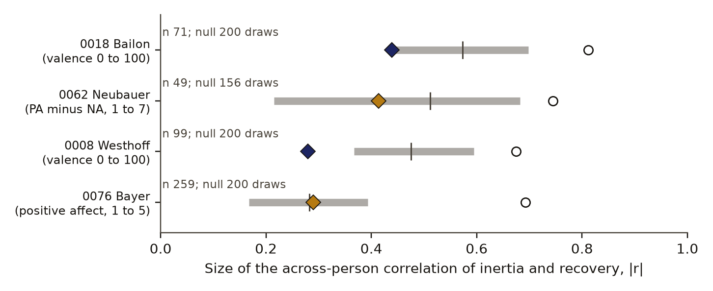
- Size of the inertia and recovery correlation in each dataset, against people simulated with one parameter.
- Chart 3
- The three rules set in advance, checked in each dataset.
- Basis
- observed: measured in this study, with a result file
c3 observed, evidence for claim 3
- Chart 3
- The three rules set in advance, checked in each dataset.
- Basis
- observed: measured in this study, with a result file
- Numbers
- None in the sentence; it reads the numbers stated beside it.
c4 observed, evidence for claim 4
- The numbers in claim 4
- 0.03; 0.47 matches the result file, 2026-11-09
- Chart 4
- Split-half reliability of each person's inertia and recovery.
- Basis
- observed: measured in this study, with a result file
c5 observed, evidence for claim 5
- The numbers in claim 5
- 0.67; 0.81 matches the result file, 2026-11-09
- Chart 1
- Correlation of inertia and recovery across people, under the planned inertia measure and the usual all-pairs one.
- Basis
- observed: measured in this study, with a result file
Introduction
Emotional inertiaDefinition: emotional inertia affective science How far a person's mood at one prompt predicts their mood at the next, measured as the lag-one correlation of their own mood series. Excludes average mood, how much mood varies, and any claim about what causes the carryover. full definition was introduced as a person-level property by Kuppens, Allen and Sheeber [2], who found higher inertia of both positive and negative emotions in people with depression and low self-esteem, across two naturalistic studies. Inertia is usually read off as an autocorrelation, so it measures how self-predictable a person's mood is from one prompt to the next.
Koval and colleagues [3] asked how inertia relates to the events people meet. In 200 first-year students, measured in daily life and in a film-clip task, the most consistent result was that higher inertia of negative affect went with slower recovery after negative stimuli. Their abstract reads this as inertia being driven mostly by weaker repair of mood after negative events. Schreuder and colleagues [5] measured recovery more directly: in a preregistered study of 68 adults with burst sampling, they timed returns to baseline after positive and negative episodes with survival analysis, and trait resilience did not predict return time.
A broader caution comes from Dejonckheere and colleagues [4]. Across many datasets, measures of mood dynamics such as autocorrelation added little to the prediction of well-being once mean affect and its variability were known. A dynamic measure has to earn its place as a separate quantity.
Our question sits between these. If inertia and recovery are two traits, they should vary across people more loosely than a model with one parameter would allow. If they are one trait, the coupling should look like what a single parameter produces on the same prompt schedules. The search we ran found adjacent work but no test of this form; that is what the search returned, not proof that none exists.
Preregistration and design
The preregistrationDefinition: preregistration research method (metascience) A dated written plan for a study, fixed and hash-locked before any result is seen: the question, the data, the statistic, the controls, the forecasts and the kill conditions. Excludes a plan revised after looking at the outcome, and a protocol written only for the record after the run. full definition was written on 29 October 2026, before any inertia, recovery, correlation or factor model was computed on the real data. Before writing it we had seen column names, row counts, the most common raw values of each mood column, and the number of prompts per person. All design choices were tested on synthetic populations first.
The idea and the prediction came from the author, who framed mood as an audio chain: a reverb, how long a feeling rings on, and a compressor release, how fast a large swing returns. The prediction had two parts, tested in each dataset separately:
- P1, separate variation: the across-person correlation of inertia and recovery has a 95 percent interval inside -0.7 to 0.7, and its size is below the 5th percentile of the same quantity from a one-parameter AR(1) null.
- P2, two factors beat one: a two-factor model of odd-day and even-day inertia and recovery beats a one-factor model, with a chi-square difference testDefinition: chi-square difference test statistics (model comparison) A test of whether a model with more free parameters fits nested data better than a simpler model, using the drop in the chi-square fit statistic against its degrees of freedom. Excludes comparisons of models that are not nested. full definition p below 0.05 and a lower BIC.
The verdictDefinition: verdict research method (our usage) The pass or fail of one preregistered rule set against the run's numbers, read off by code. Excludes an interpretation written after reading the numbers. full definition rules were fixed in advance. A dataset is "supported" when the shuffle check P0, P1 and P2 all pass; "partly" when P0 passes and exactly one of P1 and P2; "null" when P0 passes and both fail; "instrument failure" when P0 fails; "untestable" with fewer than 30 eligible people. There was no pooling across datasets, because their scales and samples differ. The preregistration's SHA-256 is given in the reproduction section.
Data and provenance
The four datasets come from openESM [1], a database of open experience samplingDefinition: experience sampling psychology (methods) A study design in which people answer short questions on a phone several times a day, so that mood is recorded close to the moment it is felt. Excludes one-off questionnaires and recall of past weeks. full definition data, all under the Creative Commons Attribution 4.0 licence (CC BY 4.0). Only group statistics are reported here; nothing describes an individual participant.
- 0018, Bailon 2020 (CoVidAffect, Spain, spring 2020): a valence slider from 0 to 100. There are no prompt numbers, so prompts are ordered by answer time and a pair needs the same day and a gap of at most 6 hours.
- 0062, Neubauer 2024 (STECCO, German first-year students, 2021): valence is the mean of four positive items minus the mean of four negative items, each 1 to 7, from the five momentary prompts a day. Two 7-day bursts six weeks apart.
- 0008, Westhoff 2024 (young adults, Germany): a valence item from 0 to 100, five prompts a day for 21 days.
- 0076, Bayer (mCog, US adults with Android phones, 2019): positive affect from 1 to 5, six prompts a day for 14 days.
The four input files were hashed by the run, and the hashes are in its result file. The samples are convenience samples, each on its own scale, which is why each is analysed alone.
Methods
Pairs, spikes and recovery
A lag pairDefinition: lag pair time-series analysis Two adjacent prompts on the same study day, the earlier one called the lead. A missed prompt or a night breaks the pair. Excludes pairs that cross a night or skip a prompt. full definition is two adjacent prompts on the same study day. For a person with mean and standard deviation over all their valid prompts, the deviation at prompt is
A spikeDefinition: spike our usage A lead prompt whose mood sits at least 1.5 of the person's own standard deviations from the person's own mean. Excludes deviations judged against other people or against a population norm. full definition is the lead prompt of a lag pair with a deviation of at least in size. For each spike, the share of the deviation that has gone at the next prompt is
clipped to the range -1 to 2. A person's recoveryDefinition: recovery affective science (our operational form) The median, over a person's spikes, of the share of each spike's distance from the person's mean that has gone by the next prompt, with 1 meaning back at the mean and 0 meaning no change. Excludes recovery measured in clock time, and recovery after events that did not produce a spike. full definition is the median of over their spikes, so 1 means back at the mean one prompt later and 0 means no change.
Inertia on disjoint pairs
Primary inertia is the Pearson rDefinition: Pearson r statistics The correlation coefficient between two quantities measured on the same units, from -1 through 0 for no linear relation to 1. Excludes non-linear relations and any statement about cause. full definition between and over the lag pairs whose lead prompt is not a spike. The reason was settled on synthetic data before the run. Inertia over all pairs is dominated by large deviations, so it reads the same spike pairs that define recovery. In a synthetic population with separate rates for small and large deviations, all-pairs inertia still correlated with recovery at -0.77 to -0.83; the disjoint version gave -0.23 to -0.29, against -0.54 to -0.61 in a one-parameter population. All-pairs inertia was kept as a secondary measure.
A person was eligible with at least 30 valid prompts, 20 lag pairs, 15 non-spike pairs and 5 spikes. A dataset was tested with at least 30 eligible people.
The across-person correlation
For each dataset, is the Pearson correlation of inertia and recovery across eligible people. Its 95 percent interval is a person bootstrapDefinition: person bootstrap statistics (resampling) An interval found by drawing people with replacement many times, recomputing the statistic each time, and taking the middle of the resulting spread. Excludes resampling of single prompts, which would treat one person's prompts as independent. full definition with 2,000 resamples.
The one-parameter null
The decisive comparison is with an AR(1) processDefinition: AR(1) process time-series statistics A series in which each value is the mean plus a fixed fraction of the previous value's distance from the mean, plus fresh random noise. The fraction is the single parameter. Excludes models with separate rates for small and large deviations, and models with measurement noise on top. full definition, in which each person has a single parameter :
where is fresh Gaussian noise. Each eligible person is simulated on their exact prompt schedule, with the same days, prompts and missed prompts, a fresh stationary start each day, their own and , and values rounded and clipped to the scale. The person's is their all-pairs inertia corrected for short-series Kendall biasDefinition: Kendall bias time-series statistics The downward bias of a lag-one correlation estimated from a short series, about (1 + 3 phi)/n for a series of n values with true value phi (Kendall 1954). Excludes bias from measurement noise, which is a separate attenuation. full definition,
with the number of pairs, then shrunk toward the dataset mean so that its spread excludes sampling noise, and clipped to -0.5 to 0.95. The whole pipeline is rerun on the simulated people, and the size of is recorded. Two hundred draws give the null distributionDefinition: null distribution statistics The spread of scores a control gives over many random draws. Its 95th percentile is the bar a real score must clear. Excludes a theoretical distribution assumed rather than drawn from the data. full definition.
The factor test
Each person gives four indicators: inertia and recovery computed on odd study days and on even study days, each half needing at least 10 non-spike pairs and 3 spikes. A one-factor modelDefinition: factor model psychometrics (confirmatory factor analysis) A model that explains the correlations among several measured indicators by a smaller number of unseen common factors, fitted by maximum likelihood. Excludes exploratory searches for the number of factors, and models of change over time. full definition (four loadings, four unique variances, 2 degrees of freedom) is compared with a two-factor model with inertia halves on one factor, recovery halves on the other and a free factor correlation (1 degree of freedom). The two-factor model wins only if the chi-square difference has p below 0.05 and its BICDefinition: BIC statistics (model selection) The Bayesian information criterion, a fit score that charges each extra parameter a penalty growing with sample size. The lower value is preferred. Excludes a test of whether either model is true. full definition is lower. The one-factor model is the two-factor model with the factor correlation at plus or minus 1, a boundary value, so the 1-degree-of-freedom p is conservative. The same halves give each measure's split-half reliabilityDefinition: split-half reliability psychometrics The correlation across people between a measure computed on one half of each person's data and the same measure on the other half. Here the halves are odd and even study days. Excludes test-retest reliability over months, and the validity of the measure. full definition.
p values from draws
Each control's p value is the share of draws at or above the real value, with one added to the count and the number of draws:
At 200 draws the smallest value is 0.005.
Controls and planted checks
Three controlsDefinition: control statistics and experimental design A version of the data with the structure under test removed (for example shuffled or pooled), scored the same way as the real data, so the real score has something to beat. Excludes a comparison with a different dataset or with a published number. full definition ran per dataset, 200 draws each, from one random generator with seed 20261029.
- C1, time shuffle: each person's mood values are permuted over their own prompt slots, and pairs and spikes are recomputed. The real mean inertia must exceed the shuffle's 95th percentile (rule P0). This checks that the instrument reads real carryover.
- C2, the one-parameter AR(1) null of eq. 3.
- C3, each person cut to a random block of 40 prompts, to see how the coupling behaves in short series.
The AR(1) null was itself a planted checkDefinition: planted check research method; called a positive control in experimental science Data built so that the right answer is known, run through the same analysis before the real data, to show that the analysis can see the effect when it is there. Excludes any check made on the real data, which cannot show what the analysis misses. full definition before the run. In a synthetic one-parameter world the observed correlation fell inside this null in 6 of 6 runs, and in a two-parameter world below its 5th percentile in 6 of 6 runs, on both continuous and 5-point scales. So the null can tell the two worlds apart when the data are as clean as the simulation.
c6 observed, evidence for claim 6
- The numbers in claim 6
- 6; 5 matches the result file, 2026-11-09
- Basis
- observed: measured in this study, with a result file
The shuffle check passed in all four datasets. Mean primary inertia was 0.236, 0.404, 0.270 and 0.162, against shuffle 95th percentiles of 0.013, 0.011, 0.013 and 0.000, each with p 0.005, the smallest value 200 draws allow.
Results
Table 1 gives the main numbers. Across people, inertia and recovery were negatively correlated in all four datasets, r -0.44, -0.41, -0.28 and -0.29. Each 95% intervalDefinition: 95% interval statistics The range that holds the middle 95 percent of the bootstrap or control draws for a number. We report it beside the number. Excludes a statement that the true value lies inside with 95 percent probability. full definition excludes 0 and lies inside -0.7 to 0.7. People whose mood carries over more tend to recover less of a spike by the next prompt.
r across people (below 0: more carryover, less recovery)
- Planned measure: inertia from pairs that are not spikes
- All-pairs inertia (shares pairs with recovery)
- 95% bootstrap interval over people
- bound, −0.7
- no relation
Data behind chart 1 4 rows
| Dataset | People | r, planned measure | 95% interval | r, all-pairs inertia | 95% interval | r, Kendall-corrected inertia | r, spike threshold 1.0 SD |
|---|---|---|---|---|---|---|---|
| 0018 | 71 | −0.44 | −0.63 to −0.19 | −0.81 | −0.87 to −0.72 | −0.43 | −0.37 (n 79) |
| 0062 | 49 | −0.41 | −0.68 to −0.09 | −0.75 | −0.86 to −0.59 | −0.42 | −0.32 (n 138) |
| 0008 | 99 | −0.28 | −0.45 to −0.09 | −0.67 | −0.78 to −0.53 | −0.28 | −0.27 (n 112) |
| 0076 | 259 | −0.29 | −0.41 to −0.15 | −0.69 | −0.76 to −0.62 | −0.29 | −0.16 (n 272) |
Read from result.json (mood study run), run 20261029T130553Z. SHA-256 of the run's file 04be61c813621f862a23b4c5006ae4579995e90ec925268ee3b2b1a5227b14d3 and of the published copy 9cf98423c63f66d0cda9e7d100c46f65a69262f220e7c7e1d7da2f539e736b34. In the copy, file paths are cut to the file name and the layout (indentation, line endings) may differ; every value is the same.
The coupling was weaker than a one-parameter AR(1) null in two datasets, 0008 clearly and 0018 by 0.001, and sat inside that null in the other two. In 0008 the size of was 0.279 against a null 5th percentile of 0.367. In 0018 it was 0.4391 against 0.4399, a pass that a different seed could reverse. In 0062 it was 0.414 inside a null running from 0.215 to 0.682, and in 0076 it was 0.289, next to the null mean of 0.283. Figure 1 draws these against the null and beside the all-pairs value.
size of r (lower: the two measures vary more separately)
- size of r in the real data
- one-parameter null, 5th to 95th percentile
- control mean
Data behind chart 2 4 rows
| Dataset | People | Size of r | Null 5th pct | Null mean | Null 95th pct | Null draws | Below the null |
|---|---|---|---|---|---|---|---|
| 0018 | 71 | 0.4391 | 0.4399 | 0.573 | 0.698 | 200 | yes |
| 0062 | 49 | 0.4138 | 0.2155 | 0.512 | 0.682 | 156 | no |
| 0008 | 99 | 0.2792 | 0.3670 | 0.475 | 0.595 | 200 | yes |
| 0076 | 259 | 0.2894 | 0.1680 | 0.283 | 0.393 | 200 | no |
Read from result.json (mood study run), run 20261029T130553Z. SHA-256 of the run's file 04be61c813621f862a23b4c5006ae4579995e90ec925268ee3b2b1a5227b14d3 and of the published copy 9cf98423c63f66d0cda9e7d100c46f65a69262f220e7c7e1d7da2f539e736b34. In the copy, file paths are cut to the file name and the layout (indentation, line endings) may differ; every value is the same.
| Rule | Value | Bar | Result |
|---|---|---|---|
| 0018: mean inertia above the shuffle's 95th percentile | 0.236 | 0.013 | holds |
| 0018: size of r below the null's 5th percentile | 0.4391 | 0.4399 | holds |
| 0018: two factors beat one, p under 0.05 | 0.81 | 0.05 | fails |
| 0062: mean inertia above the shuffle's 95th percentile | 0.404 | 0.011 | holds |
| 0062: size of r below the null's 5th percentile | 0.4138 | 0.2155 | fails |
| 0062: two factors beat one, p under 0.05 | not fitted | 0.05 | untestable |
| 0008: mean inertia above the shuffle's 95th percentile | 0.270 | 0.013 | holds |
| 0008: size of r below the null's 5th percentile | 0.2792 | 0.3670 | holds |
| 0008: two factors beat one, p under 0.05 | 0.97 | 0.05 | fails |
| 0076: mean inertia above the shuffle's 95th percentile | 0.162 | −0.00002 | holds |
| 0076: size of r below the null's 5th percentile | 0.2894 | 0.1680 | fails |
| 0076: two factors beat one, p under 0.05 | 1.00 | 0.05 | fails |
Data behind chart 3 12 rows
| Rule | Value | Bar | Result |
|---|---|---|---|
| 0018: mean inertia above the shuffle's 95th percentile | 0.236 | 0.013 | holds |
| 0018: size of r below the null's 5th percentile | 0.4391 | 0.4399 | holds |
| 0018: two factors beat one, p under 0.05 | 0.81 | 0.05 | fails |
| 0062: mean inertia above the shuffle's 95th percentile | 0.404 | 0.011 | holds |
| 0062: size of r below the null's 5th percentile | 0.4138 | 0.2155 | fails |
| 0062: two factors beat one, p under 0.05 | not fitted | 0.05 | untestable |
| 0008: mean inertia above the shuffle's 95th percentile | 0.270 | 0.013 | holds |
| 0008: size of r below the null's 5th percentile | 0.2792 | 0.3670 | holds |
| 0008: two factors beat one, p under 0.05 | 0.97 | 0.05 | fails |
| 0076: mean inertia above the shuffle's 95th percentile | 0.162 | −0.00002 | holds |
| 0076: size of r below the null's 5th percentile | 0.2894 | 0.1680 | fails |
| 0076: two factors beat one, p under 0.05 | 1.00 | 0.05 | fails |
Read from result.json (mood study run), run 20261029T130553Z. SHA-256 of the run's file 04be61c813621f862a23b4c5006ae4579995e90ec925268ee3b2b1a5227b14d3 and of the published copy 9cf98423c63f66d0cda9e7d100c46f65a69262f220e7c7e1d7da2f539e736b34. In the copy, file paths are cut to the file name and the layout (indentation, line endings) may differ; every value is the same.
A factor model with two factors never fit better than one. In 0018 (53 people with both halves) the chi-square difference was 0.055 with p 0.81 and the BIC favoured one factor by 3.9; the factor correlation was 0.95. In 0008 (60 people) the difference was 0.001 with p 0.97, BIC +4.1, factor correlation 0.98. In 0076 (152 people) the difference was 0.00 with p 1.0, BIC +5.0, and the factor correlation sat at the boundary, -1.00. In 0062 only 5 people had enough spikes on both odd and even days, because the study ran in two 7-day bursts, so the model could not be fitted.
Split-half reliability ran from 0.03 to 0.47, so the factor test had little power. For inertia it was 0.38, 0.47 and 0.03 in 0018, 0008 and 0076; for recovery 0.33, 0.11 and 0.17. Two factors cannot separate when each indicator carries this much noise.
The definition of inertia matters more than any other choice. With the usual all-pairs inertia, which reuses the spike pairs, the correlation reached 0.67 to 0.81 in size. The values were -0.81, -0.75, -0.67 and -0.69. Under that definition P1 would have failed in every dataset on its first condition. Other preregistered sensitivity checks changed no conclusion: Kendall-corrected inertia gave r -0.43, -0.42, -0.28 and -0.29, and a spike threshold of 1.0 standard deviations gave -0.37, -0.32, -0.27 and -0.16 with more people eligible (79, 138, 112 and 272).
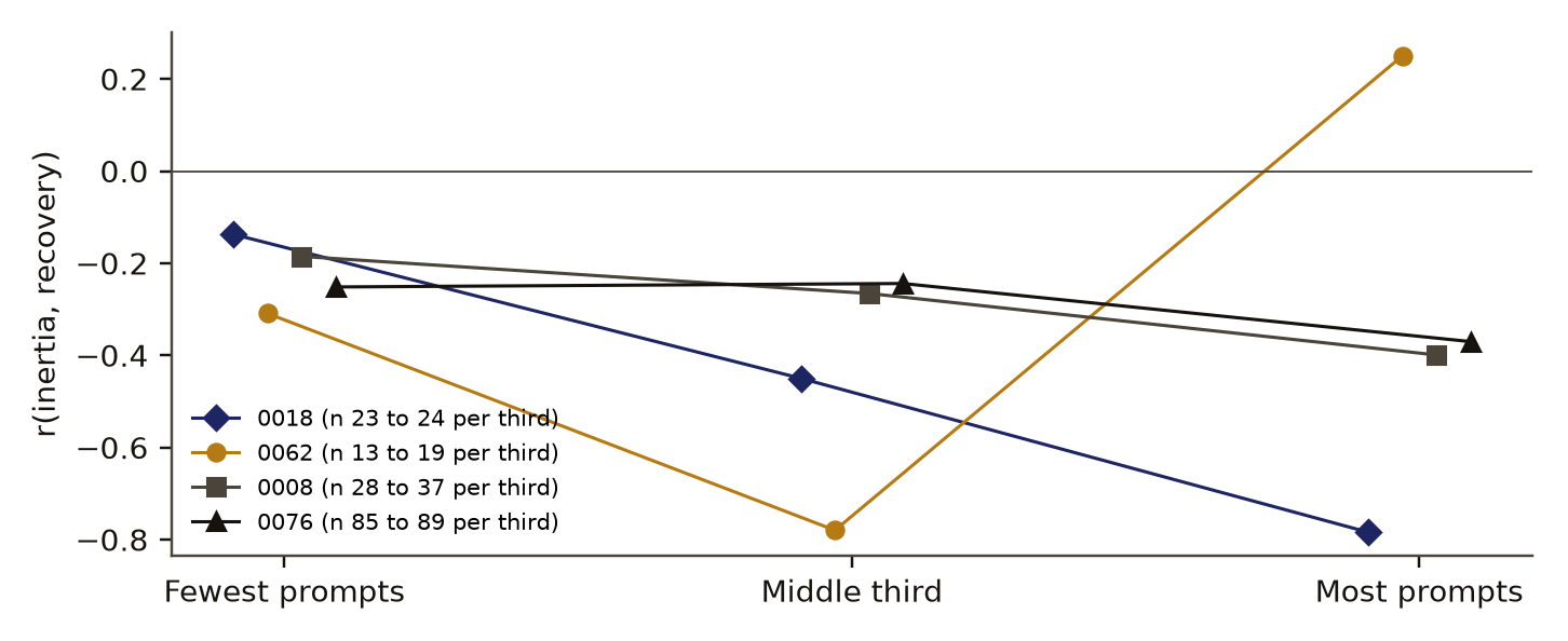
Coupling grew with series length in three datasets (Figure 2). Split by prompts per person into thirds, ran -0.14, -0.45 and -0.78 in 0018, -0.19, -0.27 and -0.40 in 0008, and -0.25, -0.24 and -0.37 in 0076. In 0062 it ran -0.31, -0.78 and +0.25 with 13 to 19 people per third. This pattern fits attenuationDefinition: attenuation psychometrics The shrinking of an observed correlation toward zero when the measures that enter it are noisy. Excludes a true weak relation between the underlying quantities. full definition: in short series both measures are noisy and the correlation shrinks toward zero. The thirds are small and have no intervals. The 40-prompt control C3 was usable only in 0076, where the mean size of was 0.235 (5th to 95th percentile 0.104 to 0.370); in the other three, too few people stayed eligible in 40 prompts.
Table 2 sets the forecasts written in the preregistration against the outcomes.
Discussion
Read by the preregistered rules, 0018 and 0008 are "partly" (P1 passed, P2 failed), 0076 is "null", and 0062 failed P1 with P2 untestable. No dataset supported both parts of the prediction. The headline is therefore that inertia and recovery were not shown to be separate traits.
That does not show they are one trait, and two features of the design lean toward a pass rather than a fail. The AR(1) null has no measurement-noise term. Noise in the real data weakens the observed coupling, which makes a real value below the null's 5th percentile easier to reach. The two P1 passes are weak evidence for that reason, and the 0018 pass sits at the edge. The factor test, on the other side, had too little reliability to detect two factors even if they exist.
The direction agrees with Koval and colleagues [3], whose abstract reports higher negative-affect inertia going with slower recovery. It also fits the caution of Dejonckheere and colleagues [4]: a dynamic measure computed from few prompts carries little information of its own, and here two such measures could not be told apart. Recovery measured in clock time with dense sampling, as in Schreuder and colleagues [5], is a better instrument for the question than one-prompt-later recovery from five or six prompts a day.
The methods result stands apart from the null. Inertia computed over all pairs shares data with recovery, and in these four datasets that overlap alone moves the size of the correlation from 0.28 to 0.44 up to 0.67 to 0.81. Any study that relates autocorrelation to recovery after peaks should compute them from disjoint pairs, or report how much of the link the overlap creates.
Limitations
- Split-half reliability was 0.03 to 0.47, so the factor test had little power, and one dataset could not be fitted at all.
- The AR(1) null has no measurement-noise term, which favours a pass on P1.
- Recovery rests on few spikes per person, and one prompt later is a coarse clock.
- The four datasets are convenience samples on different scales and items, and three of the four eligible samples are small.
- The 40-prompt control was usable in one dataset only.
- A second round with a noise term was preregistered on the same day. No run of it is on record, so its outcome is unknown.
- Scoring was done by our own code and was not blind.
Evidence
Honest null. Split-half reliability ran from 0.03 to 0.47, so the factor test had little power; two separate traits are not ruled out.
Figures
These are the paper's own figures, numbered as in the PDF, and each "Figure" reference in the text points here. The charts on this page redraw the same results from the result files and carry their own numbers.
Tables
| Dataset | Eligible | r (95% interval) | Null 5th pct, mean | P1 | Factor r |
|---|---|---|---|---|---|
| 0018 | 71 of 999 | -0.44 (-0.63 to -0.19) | 0.440, 0.573 | pass | 0.95 |
| 0062 | 49 of 321 | -0.41 (-0.68 to -0.09) | 0.215, 0.512 | fail | untestable |
| 0008 | 99 of 114 | -0.28 (-0.45 to -0.09) | 0.367, 0.475 | pass | 0.98 |
| 0076 | 259 of 519 | -0.29 (-0.41 to -0.15) | 0.168, 0.283 | fail | -1.00 |
| Quantity | Forecast | Outcome |
|---|---|---|
| Shuffle check P0 passes in every tested dataset | probability 0.9 | 4 of 4 |
| Mean primary inertia between 0.10 and 0.40 | each dataset | 3 of 4 (0062: 0.404) |
| r negative, about -0.2 to -0.5 | each dataset | 4 of 4 |
| 95% interval inside -0.7 to 0.7 | probability 0.8 each | 4 of 4 |
| Size of r below the AR(1) null 5th percentile | probability 0.35 each | 2 of 4 |
| Two factors beat one | probability 0.3 each | 0 of 3 tested |
| Split-half reliability of recovery 0.1 to 0.3 | expected | 2 of 3 (0.33, 0.11, 0.17) |
| 0018 untestable or thin | probability 0.4 | tested, 71 people |
Appendix A. The preregistered verdicts
Each verdict is a set of rules written before the run, read off by code. Values are from the run's result file. P0 compares mean inertia with the shuffle's 95th percentile; P1 compares the size of r with the AR(1) null's 5th percentile (its interval conditions held everywhere); P2 needs a chi-square difference p below 0.05 and a lower two-factor BIC; S needs the 40-prompt control's mean size of r below 0.7.
| Rule | 0018 | 0062 | 0008 | 0076 |
|---|---|---|---|---|
| P0 | pass: 0.236 over 0.013 | pass: 0.404 over 0.011 | pass: 0.270 over 0.013 | pass: 0.162 over 0.000 |
| P1 | pass: 0.439 under 0.440 | fail: 0.414 over 0.215 | pass: 0.279 under 0.367 | fail: 0.289 over 0.168 |
| P2 | fail: p 0.81, BIC +3.9 | untestable: 5 people | fail: p 0.97, BIC +4.1 | fail: p 1.0, BIC +5.0 |
| S | untestable | untestable | untestable | pass: 0.235 |
| Reading | partly | P1 null, P2 untestable | partly | null |
Numbers recorded in our publication register
| What | Value |
|---|---|
| Sample | 4 datasets: n 71, 49, 99, 259 |
| Main estimate and interval | r -0.44, -0.41, -0.28, -0.29; for dataset 0018 the interval is -0.63 to -0.19 |
| Forecast against outcome | separate variation passed in 2 of 4 datasets; two factors beating one passed in none |
| Known-answer check | the time-shuffle control passed in all 4 datasets |
As recorded in the publication register, the summary row each finding gets; the paper's own numbers above were re-read from the result files.
What lowers it
- blinding Not blind: the analyst saw the data's shape before the lock. from our publication register, on blinding
- imprecision Split-half reliability ran from 0.03 to 0.47, so the factor test had little power; two separate traits are not ruled out. from the bound stated under Evidence
- depth of reading The cited literature was read at the level of abstracts and publisher or repository pages; full texts were not read. from the Verified section
What holds it up
- scoring Scored by code against rules fixed in advance. from our publication register, on who scored it
- preregistration Preregistered and hash-locked before the run (sha256 c26b85b5). from the Reproduce section
- control Controls: the time shuffle removes inertia, as it should; the one-parameter null has no noise term. from our publication register, on controls
- open data Public data. from our publication register, on the data licence
Where the claim stands
- lead
- hypothesis
- thesis
- conjecture
- theorem
- law candidate
- killed
The two-trait model never beat the one-trait model in the three datasets where both were fitted, so the claim failed its own test. The measures were unreliable enough that the test had little power, and two separate traits are not ruled out. Tier D: Reported as a null. Power is limited by split-half reliability of 0.03 to 0.47, and the null has no noise term, so it does not show a single trait.
Trail
Versions
- v3 2026-11-09, paper version 1.0, first published PDF sha256 d09dea91f6a8d1b4
- v2 2026-10-31, dated correction, 1 item
- v1 2026-10-29, entered in the findings ledger
Corrections
2026-11-09 number found by the publication pass
The study's notes give 24 people per third in 0018; the result file gives 24, 23 and 24, which this paper uses.
2026-10-31 wording found by a review of our findings ledger
A review of our ledger noted that the F27 entry named no result file. now The result file exists and is the source of every number in this paper.
Each correction is a dated note; the findings ledger is never rewritten, and a note governs where it differs.
Ledger and version dates up to publication are local dates in US Pacific time. Clock times in the text are UTC, seven or eight hours ahead, so a lock or a run stamped just after midnight UTC belongs to the previous local day. Corrections from 14 November 2026 on are dated in UTC.
References
- Siepe, B. S., Haslbeck, J. M. B., Kloft, M., Büchner, A., Zhang, Y., Fried, E. I. and Heck, D. W. (2026). Introducing openESM: a database of openly available experience sampling datasets. Behavior Research Methods 58, 240. doi:10.3758/s13428-026-03112-y. Datasets 0018, 0062, 0008 and 0076, CC BY 4.0. run here Licence: openESM CC BY 4.0 used in Data and provenance
- Kuppens, P., Allen, N. B. and Sheeber, L. B. (2010). Emotional inertia and psychological maladjustment. Psychological Science 21, 984-991. doi:10.1177/0956797610372634 abstract or summary, 2026-11-09: abstracts and publisher or repository pages; full text not read used in Introduction
- Koval, P., Brose, A., Pe, M. L., Houben, M., Erbas, Y., Champagne, D. and Kuppens, P. (2015). Emotional inertia and external events: the roles of exposure, reactivity, and recovery. Emotion 15, 625-636. doi:10.1037/emo0000059 abstract or summary, 2026-11-09: abstracts and publisher or repository pages; full text not read used in Introduction, Discussion
- Dejonckheere, E., Mestdagh, M., Houben, M., Rutten, I., Sels, L., Kuppens, P. and Tuerlinckx, F. (2019). Complex affect dynamics add limited information to the prediction of psychological well-being. Nature Human Behaviour 3, 478-491. doi:10.1038/s41562-019-0555-0 abstract or summary, 2026-11-09: abstracts and publisher or repository pages; full text not read used in Introduction, Discussion
- Schreuder, M. J., Ariens, S., Lafit, G. and Ceulemans, E. (2024). Bouncing back from emotional ups and downs: insights in emotional recovery using survival analyses of burst ESM data. Cognition and Emotion 39, 910-919 (online 2024). doi:10.1080/02699931.2024.2423706 abstract or summary, 2026-11-09: abstracts and publisher or repository pages; full text not read used in Introduction, Discussion
- Kendall, M. G. (1954). Note on bias in the estimation of autocorrelation. Biometrika 41, 403-404. doi:10.1093/biomet/41.3-4.403 abstract or summary, 2026-11-09: abstracts and publisher or repository pages; full text not read listed, not cited in the text
Cited by later findings
- No later record in the findings ledger treats this finding.
Reproduce
Data
- Siepe 2026. Licence: openESM CC BY 4.0. https://doi.org/10.3758/s13428-026-03112-y
Preregistration
sha256 c26b85b57ec1c6495ee297009a4f7fa1e47184cfa1ee10b4aba77cef4280ce81
plan 86d93b056d781b181f3873196c9a1ac049d019b151c230a16de2693e0ff51201
Steps
- Data: download openESM datasets 0018, 0062, 0008 and 0076 (CC BY 4.0).
- For each person, form lag pairs of adjacent prompts on the same day, flag spikes at 1.5 standard deviations from the person's mean, and compute recovery with eq. 2 and inertia over non-spike pairs.
- Correlate inertia and recovery across eligible people with a 2,000-resample person bootstrap.
- Run the time shuffle, the AR(1) null of eqs. 3 and 4, and the 40-prompt blocks, 200 draws each, seed 20261029.
- Fit one-factor and two-factor models to odd-day and even-day halves.
- Preregistration SHA-256: c26b85b57ec1c6495ee297009a4f7fa1e47184cfa1ee10b4aba77cef4280ce81. Plan SHA-256: 86d93b056d781b181f3873196c9a1ac049d019b151c230a16de2693e0ff51201. Run 20261029T130553Z.
Cost. The timings in the result file sum to about 63 seconds on one desktop CPU. The study was not re-run for this paper.
Downloads
- Whitepaper, PDF F27.pdf, 558 KB
- BuildTeX source F27.bld, 34 KB
- Build receipt F27.buildtex.json, 1 KB
- BuildLang doc module doc.bld, 5 KB, imported by the source
The PDF is typeset by BuildTeX from F27.bld, which is written from the same source as this page. The receipt records the source's SHA-256 and the PDF's (d09dea91f6a8), so anyone can rebuild it and compare. The copy here has its hidden author field blanked, as the site does for every file it publishes; blank the same field in a rebuild before comparing. The name stays on the first page.
Verified
Verified on 2026-11-09. On 9 November 2026 the person counts, the four correlations with their intervals, the shuffle and AR(1) null quantiles and draw counts, the factor-model statistics and correlations, the split-half reliabilities, the all-pairs, Kendall-corrected and 1.0 standard deviation correlations, and the tertile values were re-read from the run's result file. They match the findings ledgerDefinition: findings ledger our records The append-only, dated list of every result we have recorded, numbered F1, F2 and on. Corrections are added as new dated lines and old entries are never rewritten. Excludes a curated list of successes. full definition entry and the study's own log. The preregistration's SHA-256 was recomputed and matches the hash recorded in the result file. The synthetic checks and the forecasts were read from the preregistration. Both figures were drawn by a script that reads only the result file. For Kendall [6] only the bibliographic record was seen, and the bias formula used here is the one written in our preregistration.
Not checked. The study was not re-run for this paper. The literature in the introduction was found by searches run on 9 November 2026 and read at the level of abstracts and publisher or repository pages; the full texts were not read.
Terms on this page
Each term is defined where it is first used on this page. Each name below opens its entry in the findings glossary, which lists every page that uses it.
- honest null research method (our usage) first use
- emotional inertia affective science first use
- preregistration research method (metascience) first use
- chi-square difference test statistics (model comparison) first use
- verdict research method (our usage) first use
- experience sampling psychology (methods) first use
- lag pair time-series analysis first use
- spike our usage first use
- recovery affective science (our operational form) first use
- Pearson r statistics first use
- person bootstrap statistics (resampling) first use
- AR(1) process time-series statistics first use
- Kendall bias time-series statistics first use
- null distribution statistics first use
- factor model psychometrics (confirmatory factor analysis) first use
- BIC statistics (model selection) first use
- split-half reliability psychometrics first use
- control statistics and experimental design first use
- planted check research method; called a positive control in experimental science first use
- 95% interval statistics first use
- attenuation psychometrics first use
- findings ledger our records first use
To report an error, name the finding, the claim number and the source on the Work page, which gives the address. Accepted corrections join the Trail with their date.