
Findings F210 Optics, colour and imaging, Computing and mathematics, Physics found 2026-10-31
In a 2D wave simulation, a stepped Luneburg lens keeps its focus with shells one wavelength thick
In a two-dimensional wave simulation, a Luneburg lens built from shells one wavelength thick keeps 0.97 to 0.99 of the focal peak of the ideal graded lens, and shells 1.67 wavelengths thick keep 0.84 to 0.97 depending on size. An earlier claim that the rim index is the harder limit did not hold: the loss came from clipping the profile, and a refitted profile keeps 0.41 of the peak at a rim index of 1.3. No sphere and no hardware were tested.
- Tier
- B, signal
- Outcome
- mixed
- Rung
- lead
- Standing
- narrowed in part: the rim index claim, at a radius of 50 wavelengths in two dimensions, F303
- Corrections
- 5, latest 2026-11-14
- Version
- v2, 2026-11-14
- Redo it
- Reproduce
Download PDF 534 KB BuildTeX source F210.bld
What this means for a reader
A lens whose index must vary smoothly sounds impossible to make, and for decades that was the stated obstacle. In this simulation the smoothness matters much less than it looks: shells about one wavelength thick focus almost as well as a perfect gradient, and thicker shells lose the focus by degrees. The second lesson is about our own first reading. A lens whose outer layers cannot reach an index of 1 looked ruined, and it was only ruined because we cut the ideal profile off and did not redesign it. A solver for the full sphere, and then a measurement on a stepped lens at microwave wavelengths, would test both results.
Objection
This is a simulation in two dimensions with a scalar field. A sphere, the other polarisation, absorption and scattering at rough shell boundaries were not modelled.
What would change the call. A solver for the full sphere, then a measurement on a stepped lens at microwave wavelengths.
From the paper's first stated limitation; our register records no separate objection.
Abstract
A Luneburg lens focuses a plane wave to a point on its far surface, and needs a refractive index that falls smoothly from 1.41 at the centre to 1 at the rim. Built lenses approximate that with shells of constant index. We asked how thick the shells can be. The study is a simulation: a scalar wave solution for a layered cylinder in two dimensions, with no sphere, no absorption and no measurement. At a radius of 50 wavelengths, 30 equal shells, each 1.67 wavelengths thick, keep 0.93 of the continuous lens's focal peak; 50 shells keep 0.99 and 10 shells keep 0.54. With shells 1.67 wavelengths thick the share is 0.84 at a radius of 25 wavelengths and 0.97 at 100; with shells 1 wavelength thick it is 0.97 and 0.99. Clipping the Luneburg profile at a minimum index destroys the focus quickly: a floor of 1.05 keeps 0.76 of the peak, 1.1 keeps 0.31, 1.2 keeps 0.09 and 1.3 keeps 0.035. We first read that as a hard limit set by the rim index. A second run the same day showed otherwise. That loss belongs to the clipping: a quadratic profile refitted to the rim index keeps 0.53 at 1.1, 0.41 at 1.3 and 0.38 at 1.5.
c1 observed, evidence for claim 1
- The numbers in claim 1
- 50; 30; 1.67; 0.93; 0.99; 10; 0.54 matches the result file, 2026-11-14
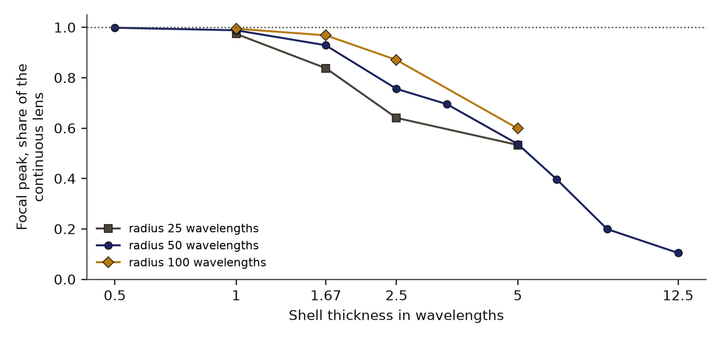
- Chart 1
- What was simulated, and what was not.
- Chart 2
- Focal peak kept by a stepped lens, by number of shells.
- Basis
- observed: measured in this study, with a result file
c2 observed, evidence for claim 2
- The numbers in claim 2
- 1.67; 0.84; 25; 0.97; 100; 1; 0.99 matches the result file, 2026-11-14
- Basis
- observed: measured in this study, with a result file
c3 observed, evidence for claim 3
- The numbers in claim 3
- 1.05; 0.76; 1.1; 0.31; 1.2; 0.09; 1.3; 0.035 matches the result file, 2026-11-14
- Chart 1
- What was simulated, and what was not.
- Chart 3
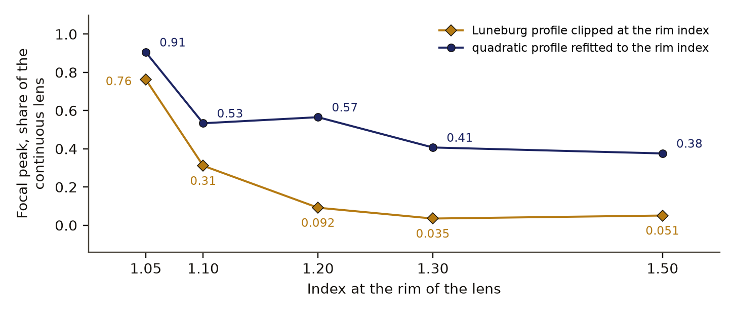
- A raised rim index: the profile clipped, and the profile refitted.
- Basis
- observed: measured in this study, with a result file
c4 observed, evidence for claim 4
- The numbers in claim 4
- 0.53; 1.1; 0.41; 1.3; 0.38; 1.5 matches the result file, 2026-11-14
- Chart 3
- A raised rim index: the profile clipped, and the profile refitted.
- Basis
- observed: measured in this study, with a result file
Introduction
The Luneburg lensDefinition: Luneburg lens optics and antenna engineering A sphere, or in two dimensions a cylinder, whose refractive index falls from the square root of 2 at the centre to 1 at the surface, so that a plane wave from any direction is focused to a point on the opposite surface. Excludes a uniform ball lens, and modified profiles whose focus lies inside or outside the surface. full definition is a sphere, or in two dimensions a cylinder, whose refractive index depends on the distance from the centre as
where is the radius. It is the best known gradient-indexDefinition: gradient-index optics Describing an optical element whose refractive index changes smoothly through the material, so that light bends inside it along curved paths. Excludes a conventional lens of one material, which bends light only at its surfaces. full definition lens, an optical element that bends light by a smooth change of index inside the material; a conventional lens, which bends light only at its surfaces, is the contrasting case. Every direction is an optical axis, so the lens has no off-axis aberration, which is why it is used as a wide-angle antenna at microwave frequencies.
No material offers that profile directly. The usual answer is the stepped lens: concentric shells, each of one index. Stepped lenses arose because graded materials were not available, and built examples often have 4 to 10 layers. Fuchs and colleagues treated the choice of shell number, thickness and index as an optimisation problem, and work citing them reports that directivity stops improving beyond a certain shell count [2]. A ray-tracing study of an optical all-sky lens considers up to 40 glass layers [3]. On the rim index, Gutman's modified Luneburg lens of 1954 moves the focus inside the sphere [4], and a later generalised profile carries the edge index as an explicit parameter, with a silicon example at an edge index of 2.2 [5].
So both of our questions have long histories in antenna engineering, and we claim nothing new. The study began from a census of instruments that were proposed and then set aside, where a 1989 patent text named the manufacture of graded material as the obstacle for gradient lenses [1]. The decision it informed was small and practical: which controls a teaching model of the lens should expose, and what numbers to put beside them. The questions were how coarse the shells can be before the focus fails, whether that depends on the size of the lens, and what happens when the outer index cannot go down to 1.
Preregistration and design
There was no preregistrationDefinition: preregistration research method (metascience) A dated written plan for a study, fixed and hash-locked before any result is seen: the question, the data, the statistic, the controls, the forecasts and the kill conditions. Excludes a plan revised after looking at the outcome, and a protocol written only for the record after the run. full definition, meaning no dated plan locked by a hash before the run, and no kill conditionDefinition: kill condition research method (our usage, after Popper's falsification) A rule written in the preregistration that, when met, decides against the claim with no room for judgement after the run. Excludes reasons found after the run for setting a result aside. full definition, an outcome fixed in advance that would end the claim. Forecasts were written to a file on 31 October 2026 before any simulation ran, and the file says so in its own first line. Three of them concern this paper: that a lens 1,000 wavelengths in radius would need 50 shells to reach the diffraction limit, that a uniform ball would be worse by a factor of 50, and that an index floor of 1.3 would break the lens (probability 0.8).
The first pass used a ray trace and gave an answer the wave solver then overturned, as the results section describes. The check of other lens sizes and the refitted rim profile were both added after the first numbers were seen. The refit had its own forecasts written before it ran: 0.6 of the peak at a rim index of 1.1 and 0.25 at 1.3.
Data and provenance
There is no external dataset. The inputs are the index profiles defined in the methods and three lens sizes. The numbers come from three result files written by the study's own Python code on 31 October 2026: the main run at a radius of 50 wavelengths, the size check at 25 and 100, and the refitted rim profile at 50.
Methods
The wave solution
The model is a cylinder of radius in vacuum, uniform along its axis, lit by a plane wave of unit amplitude with its electric field along the axis. This is a scalar problem in two dimensions. The field is written as a sum of angular orders , and for each order the radial part obeys
with the wavenumber in vacuum and the index at radius . The code integrates eq. 2 outward from near the axis with a fourth-order Runge-Kutta scheme, 120 steps per wavelength of radius, and matches the result at the surface to the incident wave plus an outgoing wave. This is the standard partial-waveDefinition: partial-wave wave physics (scattering theory) Describing a solution in which the field around a round object is written as a sum of angular orders, each order is solved along the radius alone, and the orders are added up. Excludes ray tracing, which follows paths and carries no wavelength, and grid methods that sample the whole field. full definition treatment of scattering by a cylinder, in which each angular order is solved by itself and the orders are summed; it includes every reflection between shells, and it is exact up to the numerical integration. Orders up to are kept.
What is read off
The intensity is computed along the rear surface of the cylinder, within 0.3 radian of the point opposite the source (0.2 radian in the size check), on a grid of 0.001 radian. Two numbers are read: the focal peakDefinition: focal peak our usage The largest intensity found on the rear surface of the lens within the arc examined, reported as a share of the same quantity for the continuous lens of the same size. Excludes the total power delivered, the gain of an antenna, and any peak that forms off the rear surface. full definition, which is the largest intensity on that arc, and the width of the peak at half its height, in wavelengths of arc. Every lens is reported as its focal peak divided by the focal peak of the continuous lens of eq. 1 at the same size.
The lenses
- Continuous: eq. 1.
- Stepped: shells of equal thickness , each with the index eq. 1 gives at the middle of the shell.
- Clipped: eq. 1 with every index below a floor raised to the floor, for floors of 1.05, 1.1, 1.2, 1.3 and 1.4. This stands for a material that cannot be made lighter than the floor.
- Refitted: a profile of the same quadratic form with the rim index fixed and the centre index free,
where is the rim index and the centre index. For each rim index the centre index was chosen with a ray trace so that rays meet at the rear surface, and the wave solver then scored the result. The centre indices came out between 1.45 and 1.72.
- Uniform: a cylinder of index 2 throughout, whose paraxial focus also falls on its rear surface.
The ray trace
The first pass traced 25 rays through stepped spheres with Snell's law at every shell boundary, for a lens taken to be 1,000 wavelengths in radius, and measured how far each ray lands from the focal point. It is reported because its answer was wrong in an instructive way.
Controls and planted checks
The known-answer check is an empty cylinder. With an index of 1 everywhere there is no lens, and the field on the surface must equal the incident plane wave, with magnitude 1. The solver returned a mean magnitude of 0.996 and a largest deviation of 0.026. That bounds the solver's error at about 2.6 percent in amplitude, or about 5 percent in intensity, at a radius of 50 wavelengths.
- dataA layered cylinder in two dimensionsA scalar wave solution for a plane wave on a cylinder of constant-index shells. No sphere, no absorption and no measurement.
- controlKnown answer: an empty cylinderWith every shell at index 1 the field should be the plane wave itself. The solver's largest deviation is 2.6 percent in amplitude.
- measurementFocal peak against the ideal lensThe peak intensity on the rear surface, as a share of the peak of the continuous Luneburg profile, and the width of that peak.
- simulation only0.93 at 30 shells, 0.99 at 50Clipping the profile at a minimum index of 1.3 keeps 0.035 of the peak; the refit run shows that loss belongs to the clipping.
Read from results.json (the simulation's result file; the luneburg block). SHA-256 of the run's file f9f6d525caa8adde2ba1bb167c1a6ac01750a46cdcadcb080d02ea342e389b37 and of the published copy 37f7673ca70da615a11f44ec724875c6726a483e87fbea68235ac0069b361e83. In the copy, file paths are cut to the file name and the layout (indentation, line endings) may differ; every value is the same.
The continuous lens is a second check: its peak falls at the point opposite the source, as the theory requires, with a width of 0.40 wavelength. The ray tracer was checked the same way; rays through the continuous profile met the focal point within 4e-7 of the radius.
No controlDefinition: control statistics and experimental design A version of the data with the structure under test removed (for example shuffled or pooled), scored the same way as the real data, so the real score has something to beat. Excludes a comparison with a different dataset or with a published number. full definition in the statistical sense applies, because the calculation has no random element.
Results
Shell thickness
At a radius of 50 wavelengths, 30 equal shells, each 1.67 wavelengths thick, keep 0.93 of the continuous lens's focal peak; 50 shells keep 0.99 and 10 shells keep 0.54. Table 1 gives all nine shell counts. The peak keeps its width of 0.40 wavelength from 10 shells upward; with fewer shells it also broadens.
With shells 1.67 wavelengths thick the share is 0.84 at a radius of 25 wavelengths and 0.97 at 100; with shells 1 wavelength thick it is 0.97 and 0.99. Thickness in wavelengths is therefore a fair first guide and is not the whole rule: at a fixed thickness the larger lens does better. With shells 2.5 wavelengths thick the shares are 0.64, 0.76 and 0.87 at radii of 25, 50 and 100 wavelengths, and with shells 5 wavelengths thick they are 0.53, 0.54 and 0.60. Figure 1 shows the three sizes.
The ray trace had pointed the other way. For a lens 1,000 wavelengths in radius it found no shell count up to 1,000 that brought the rays within the diffraction radius: at 1,000 shells the root-mean-square miss was 0.0098 of the radius against a diffraction radius of 0.00061. At that size 1,000 shells are 1 wavelength thick, which is where the wave solution keeps 0.97 to 0.99 of the peak at the three sizes it was run. Tracing rays through layers about one wavelength thick is outside the range where ray optics holds. The wave solver was not run at a radius of 1,000 wavelengths, so the forecast of 50 shells at that size was not tested at its own size.
A uniform cylinder of index 2 at the same size reaches 0.14 of the peak. That is a factor of 7 below the continuous lens, against a forecast factor of 50.
c5 observed, evidence for claim 5
- The numbers in claim 5
- 2; 0.14 matches the result file, 2026-11-14
- Basis
- observed: measured in this study, with a result file
::pagebreak
The rim index
Clipping the Luneburg profile at a minimum index destroys the focus quickly: a floor of 1.05 keeps 0.76 of the peak, 1.1 keeps 0.31, 1.2 keeps 0.09 and 1.3 keeps 0.035. At a floor of 1.3 the peak is 5.3 wavelengths wide. At 1.4 the largest intensity is no longer opposite the source.
That loss belongs to the clipping: a quadratic profile refitted to the rim index keeps 0.53 at 1.1, 0.41 at 1.3 and 0.38 at 1.5. The refitted lenses keep a narrow focus, 0.4 to 0.6 wavelength wide. Table 3 and Figure 2 set the two side by side. The refitted profile still loses about half the peak once the rim index reaches 1.1, so a raised rim has a cost; it is a far smaller one than the clipped numbers suggested.
Discussion
The shell result has a plain physical reading. A wave averages over structure finer than its wavelength, so steps about a wavelength thick act much like the gradient they replace, and the focus degrades smoothly as the steps grow. A ray has no wavelength and sees every step as a prism, which is why the ray trace kept reporting failure. For a lens tens of wavelengths across, the number of shells that matters is set by the wavelength and to a lesser degree by the size.
The rim result is a correction to ourselves. The first entry in our ledger said the rim index was the harder limit, on the strength of the clipped profile. Clipping leaves the inner part of the lens designed for a rim that is no longer there. Refitting the same simple form to the new rim recovers a sharp focus at about 0.4 to 0.6 of the peak for rim indices of 1.1 and above, with no optimisation at the wave level. The literature we found afterwards treats lenses with a rim index above 1 as a known family, so the refit rediscovers a small part of it.
For the teaching model the outcome was two controls: a shell count, and an edge index that redesigns the profile and does not cut it.
Limitations
- This is a simulation in two dimensions with a scalar field. A sphere, the other polarisation, absorption and scattering at rough shell boundaries were not modelled.
- The field was read only on the rear surface. A stepped or refitted lens may focus slightly inside or outside that surface, and the peak share would then understate it.
- The solver's own error is about 2.6 percent in amplitude by the empty-cylinder check, so peak shares closer than about 0.05 to each other should not be ranked.
- Widths are read on a grid of 0.05 wavelength and are coarse.
- Shells have equal thickness and mid-shell indices. No shell design was optimised, so a designed lens with the same count could do better.
- The refitted centre index was chosen by a ray trace at one size, and only one size was run for the rim results.
- The size check and the refit were added after first results were seen, and there was no preregistration.
- The ray trace and the wave solver were run at different lens sizes, so their disagreement is argued from shell thickness and was not shown at one size.
- The literature was read at the level of search snippets, and the results are likely to be known in antenna engineering.
- Scoring was by our own code and was not blind. Nobody outside the project has checked it.
Evidence
Mixed. The statement that the rim index is the harder limit did not hold. Clipping the profile keeps 0.31 of the peak at a rim index of 1.1 and 0.035 at 1.3; a quadratic profile refitted to the rim keeps 0.53 and 0.41. The forecast of a factor of 50 for a uniform cylinder missed (factor of 7), and the forecast of 50 shells for a lens 1,000 wavelengths in radius was not tested at that size.
Figures
These are the paper's own figures, numbered as in the PDF, and each "Figure" reference in the text points here. The charts on this page redraw the same results from the result files and carry their own numbers.
Tables
| Shells | Thickness, wavelengths | Peak share | Width, wavelengths |
|---|---|---|---|
| 4 | 12.5 | 0.10 | 1.2 |
| 6 | 8.33 | 0.20 | 0.9 |
| 8 | 6.25 | 0.40 | 0.5 |
| 10 | 5.0 | 0.54 | 0.4 |
| 15 | 3.33 | 0.70 | 0.4 |
| 20 | 2.5 | 0.76 | 0.4 |
| 30 | 1.67 | 0.93 | 0.4 |
| 50 | 1.0 | 0.99 | 0.4 |
| 100 | 0.5 | 1.00 | 0.4 |
| Thickness, wavelengths | Radius 25 | Radius 50 | Radius 100 |
|---|---|---|---|
| 5.0 | 0.53 (5 shells) | 0.54 (10 shells) | 0.60 (20 shells) |
| 2.5 | 0.64 (10 shells) | 0.76 (20 shells) | 0.87 (40 shells) |
| 1.67 | 0.84 (15 shells) | 0.93 (30 shells) | 0.97 (60 shells) |
| 1.0 | 0.97 (25 shells) | 0.99 (50 shells) | 0.99 (100 shells) |
| Rim index | Clipped, peak share | Clipped, width | Refitted, peak share | Refitted, width |
|---|---|---|---|---|
| 1.05 | 0.76 | 0.4 | 0.91 | 0.4 |
| 1.1 | 0.31 | 0.7 | 0.53 | 0.5 |
| 1.2 | 0.09 | 2.0 | 0.57 | 0.5 |
| 1.3 | 0.035 | 5.3 | 0.41 | 0.6 |
| 1.5 | 0.05 | 19.8 | 0.38 | 0.6 |
Appendix A. Forecasts against outcomes
The forecasts were written to files before each run. The first three come from the main forecast file and the last two from the forecast file of the refit.
| Quantity | Forecast | Outcome |
|---|---|---|
| Shells for the diffraction limit, radius 1,000 wavelengths | 50 | not tested at that size; 30 shells keep 0.93 at radius 50 |
| Uniform cylinder against the Luneburg lens | worse by a factor of 50 | worse by a factor of 7 at radius 50 |
| A floor of 1.3 breaks the lens | probability 0.8 | clipped 0.035; refitted 0.41 |
| Refitted profile, rim 1.1 | 0.6 | 0.53 |
| Refitted profile, rim 1.3 | 0.25 | 0.41 |
Numbers recorded in our publication register
| What | Value |
|---|---|
| Sample | 9 shell counts at a radius of 50 wavelengths, with radii of 25 and 100 as a size check |
| Main estimate and interval | none; the solver's own error is about 2.6 percent in amplitude |
| Forecast against outcome | Missed: a factor of 50 for a uniform cylinder (the run gave 7). Withdrawn: the rim index as the harder limit, after a refitted profile kept 0.41 of the peak at a rim index of 1.3 |
| Known-answer check | an empty cylinder, which the solver reproduces within 2.6 percent in amplitude |
As recorded in the publication register, the summary row each finding gets; the paper's own numbers above were re-read from the result files.
What lowers it
- blinding Not blind. No preregistration; the size check and the refit were added after first results were seen. from our publication register, on blinding
- depth of reading The cited literature was read at the level of search snippets; full texts were not read. from the Verified section
What holds it up
- scoring Scored by code against rules fixed in advance. from our publication register, on who scored it
- control Controls: none beyond the empty-cylinder known-answer check. from our publication register, on controls
Where the claim stands
- lead
- hypothesis
- thesis
- conjecture
- theorem
- law candidate
- killed
An observation with a source. No prediction with a kill condition was on file before the run, which the next rung needs. Tier B: A clean known answer for the ideal lens, in two dimensions only; the result is likely known in antenna engineering.
Trail
Versions
- v2 2026-11-14, paper version 1.0, first published PDF sha256 7b8033f38c7c24d8
- v1 2026-10-31, entered in the findings ledger
Corrections
2026-11-14 wording found by the publication pass
The word "exact" in the ledger title is replaced by a description of the solver with its measured error.
2026-11-14 scope found by the publication pass
The ledger entry's figure for the field angle at which a parabola's coma reaches the diffraction limit is left out, because it rests on a formula entered from memory.
2026-11-14 scope found by the publication pass
Narrowed the claim to shell thickness and to the clipped profile as a design error, because the rim limit in the ledger title did not survive the refit.
2026-10-31 retraction found by the study itself, before publication
A later ledger entry, F303, found that the loss at a raised rim index came from clipping the profile. now A refitted quadratic profile keeps 0.53 of the peak at a rim index of 1.1 and 0.41 at 1.3, where clipping keeps 0.31 and 0.035. The statement that the rim index is the harder limit was withdrawn.
2026-10-31 wording found by the study itself, before publication
A first pass by ray trace found that no shell count up to 1,000 reached the diffraction limit. now The wave solution replaced it the same day.
Standing, and the ledger entries it rests on
2026-10-31 narrowed in part F303
Set by hand from findings ledger entry F303, dated 2026-10-31: the rim index claim, at a radius of 50 wavelengths in two dimensions. Rests on findings ledger, F303.
Each correction is a dated note; the findings ledger is never rewritten, and a note governs where it differs.
Ledger and version dates up to publication are local dates in US Pacific time. Clock times in the text are UTC, seven or eight hours ahead, so a lock or a run stamped just after midnight UTC belongs to the previous local day. Corrections from 14 November 2026 on are dated in UTC.
References
- Suzuki, M. and Hattori, J. (1989). Gradient index lens. United States Patent 4,848,882. abstract or summary, 2026-11-14: search snippets; full text not read used in Introduction
- Fuchs, Le Coq, Lafond, Rondineau and Himdi. Design optimization of multishell Luneburg lenses. IEEE Transactions on Antennas and Propagation. abstract or summary, 2026-11-14: search snippets; full text not read used in Introduction
- Modeling of a stepped Luneburg lens for all-sky surveys (2018). arXiv:1806.05661. abstract or summary, 2026-11-14: search snippets; full text not read used in Introduction
- Gutman, A. S. (1954). Modified Luneburg lens. Journal of Applied Physics 25, 855-859. abstract or summary, 2026-11-14: search snippets; full text not read used in Introduction
- Ultrashort waveguide tapers based on Luneburg lens (2019). arXiv:1910.11281. abstract or summary, 2026-11-14: search snippets; full text not read used in Introduction
Cited by later findings
- F303 narrowed in part, the rim index claim, at a radius of 50 wavelengths in two dimensions, 2026-10-31 (record findings ledger, F303). A quadratic profile refitted to the rim index keeps 0.53 of the focal peak at rim 1.1, 0.41 at 1.3 and 0.38 at 1.5, where clipping keeps 0.31, 0.035 and 0.05, so the rim limit in F210 came from the clipping.
Reproduce
Steps
- Data: no external dataset. The inputs are the index profiles in the Methods section; the simulation code is not yet in a public repository.
- For each angular order up to , integrate eq. 2 from 0.001 of the radius to the surface with 120 Runge-Kutta steps per wavelength of radius, and match to Bessel and Hankel functions outside.
- Sum the orders on the rear surface, take the largest intensity and its width at half height, and divide the peak by that of eq. 1.
- Repeat for stepped profiles of 4 to 100 shells at a radius of 50 wavelengths, for thicknesses of 5, 2.5, 1.67 and 1 wavelengths at radii of 25 and 100, for clipped profiles, for eq. 3, for an index of 2 and for an index of 1.
- No preregistration exists, so there is no preregistration hash, plan hash or run id. The forecast files carry a written date and no hash. The wave calculation uses no random numbers.
Cost. The main run, ray trace included, took about 18 s on one desktop CPU. The simulation was not re-run for this paper.
Downloads
- Whitepaper, PDF F210.pdf, 534 KB
- BuildTeX source F210.bld, 28 KB
- Build receipt F210.buildtex.json, 1 KB
- BuildLang doc module doc.bld, 5 KB, imported by the source
The PDF is typeset by BuildTeX from F210.bld, which is written from the same source as this page. The receipt records the source's SHA-256 and the PDF's (7b8033f38c7c), so anyone can rebuild it and compare. The copy here has its hidden author field blanked, as the site does for every file it publishes; blank the same field in a rebuild before comparing. The name stays on the first page.
Verified
Verified on 2026-11-14. On 14 November 2026 every peak share and width in the three tables, the empty-cylinder check, the continuous lens's width, the uniform cylinder's share and the ray-trace misses were re-read from the main result file; the shares at radii of 25 and 100 wavelengths from the size-check file; and the clipped and refitted shares, widths and centre indices from the refit's result file. They match the findings ledgerDefinition: findings ledger our records The append-only, dated list of every result we have recorded, numbered F1, F2 and on. Corrections are added as new dated lines and old entries are never rewritten. Excludes a curated list of successes. full definition and its later entry on the refit. The forecasts were re-read from the two forecast files. The solver's equations, step counts and grids were read from its source code. Both figures were drawn by a script that reads only those result files.
Not checked. The simulation was not re-run for this paper. The literature was found by two searches on 14 November 2026 and read at the level of search snippets; the full texts were not read, and the reference to Fuchs and colleagues is given without year or volume because the search results did not show them.
Terms on this page
Each term is defined where it is first used on this page. Each name below opens its entry in the findings glossary, which lists every page that uses it.
- Luneburg lens optics and antenna engineering first use
- gradient-index optics first use
- preregistration research method (metascience) first use
- kill condition research method (our usage, after Popper's falsification) first use
- partial-wave wave physics (scattering theory) first use
- focal peak our usage first use
- control statistics and experimental design first use
- findings ledger our records first use
To report an error, name the finding, the claim number and the source on the Work page, which gives the address. Accepted corrections join the Trail with their date.