
Findings F172 Psychology and perception, Method and statistics found 2026-10-31
A selection model shrinks the overstatement in published effects but cannot pick which replicate
Fitted to published original results from other fields, a model that accounts for the significance filter predicted replication far better than taking originals at face value. In a held-out field it did no better than the plain base rate, and a small logistic model beat it.
- Tier
- B, signal
- Outcome
- mixed
- Rung
- hypothesis
- Verdicts
- 5 passed, 4 failed
- Kill rule
- fired
- Corrections
- 2, latest 2026-11-14
- Version
- v3, 2026-11-14
- Redo it
- Reproduce
Download PDF 601 KB BuildTeX source F172.bld
What this means for a reader
If a published effect cleared p below 0.05, expect a replication to find it smaller, and expect the chance of a successful replication to be well below what the original's own numbers imply. A model of the significance filter turns that expectation into a number that is far better than trusting the original. It does not tell you which single finding will hold. On these data the plain original z value, read through a small regression, is the stronger tool for picking claims to check.
Objection
Fisher z standard errors ignore design, and unsigned rows assume direction.
What would change the call. Lock the two-normal prior and review the conversions by hand on a sample.
From the strongest objection recorded in our publication register.
Abstract
Published effects that cleared a significance threshold tend to be overstated, and replications of them succeed less often than their own statistics suggest. We asked whether one model of that filter, fitted only to the significant originals of other fields, can predict which effects replicate in a field it has not seen. On 1,222 significant originals in 307 replication projects, pooled from the Reproducibility Project Psychology and the FORRT Replication Database, each of eight fields was held out in turn and forecasts were scored by Brier score. The selection model beat taking the originals at face value by 0.142 in Brier score (95% interval 0.108 to 0.186) and did not beat the base rate, at -0.004 (-0.039 to 0.027). A small logistic model on the original z value and the two sample sizes beat the selection model by 0.037 (0.011 to 0.069). The preregistered kill rule fired, and the claim that the model tells which effects replicate is withdrawn. The reading that significant originals are inflated survives on these data.
c1 observed, evidence for claim 1
- The numbers in claim 1
- 0.142; 95; 0.108; 0.186; -0.004; -0.039; 0.027 matches the result file, 2026-11-09
- Chart 2
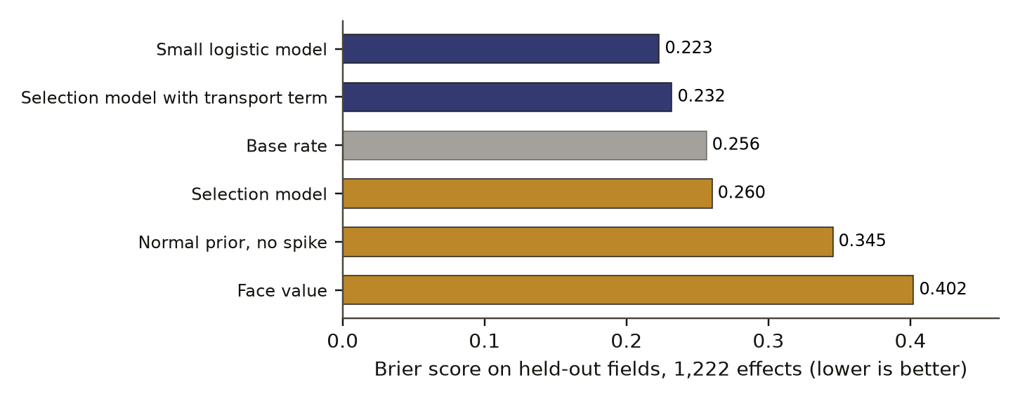
- Held-out Brier score of six forecasts of which effects replicate.
- Basis
- observed: measured in this study, with a result file
c2 observed, evidence for claim 2
- The numbers in claim 2
- 0.037; 0.011; 0.069 matches the result file, 2026-11-09
- Chart 3
- The four comparisons set in advance: each competitor's Brier score minus the selection model's.
- Basis
- observed: measured in this study, with a result file
Introduction
The Open Science Collaboration [1] repeated 100 studies from three psychology journals and found that far fewer replications than originals reached significance. Since then, replication results have been gathered into databases. The FORRT Replication Database, FReD, joins earlier collections and pairs original findings with their replications at the level of single effects [4].
One explanation of the gap needs no misconduct. When results are published only if significant, the significance filterDefinition: significance filter (winner's curse) metascience and statistics The selection of published results by a significance threshold, which lets lucky overestimates through more often than underestimates, so the published effects of a set of studies are on average larger than the true ones. Excludes deliberate misconduct, which the filter neither requires nor detects. full definition lets through estimates that happened to land high. Gelman and Carlin [5] named the two resulting errors: the sign of a significant estimate can be wrong (Type S), and its size can be exaggerated (Type M), and both grow as power falls. A replication of the same size then succeeds less often than the original's estimate predicts.
Two families of tools forecast replication. Statistical models of selection, such as z-curve [6], fit the distribution of significant z values and estimate how often exact replications should succeed. Learned models predict from features of the original; Altmejd and colleagues [7] trained such a model on replications in economics and psychology and found, among other things, that interaction effects replicate worse than main effects.
This paper puts a selection modelDefinition: selection model meta-analysis and statistics A model of observed results that writes down both a distribution of true effects and the rule by which results get seen, here the rule that only originals with z above 1.96 in absolute value are seen, and fits both together. Excludes a model that takes the observed results as an unselected sample. full definition in a held-out test against three baselines, with all parameters fitted away from the field being forecast. The question is narrow: does a model of the filter pick out which effects replicate, or does it only set the level? Our search did not find a test of this exact design. That is what the search returned, and it does not show that none exists.
Preregistration and design
The design was written as a preregistrationDefinition: preregistration research method (metascience) A dated written plan for a study, fixed and hash-locked before any result is seen: the question, the data, the statistic, the controls, the forecasts and the kill conditions. Excludes a plan revised after looking at the outcome, and a protocol written only for the record after the run. full definition and hash-locked on 31 October 2026 at 08:21 UTC, before any replication outcome was scored. Seen before the lock: column names, counts by category, the number of original statistics that could be converted, and outcomes simulated by the code. The published replication rate of the Reproducibility Project, 36 percent, was known, so the forecast for that field was not blind to its headline.
The locked file names the data, the conversions, the model, the held-out scheme, the baselines, the score, the interval and test methods, the planted checkDefinition: planted check research method; called a positive control in experimental science Data built so that the right answer is known, run through the same analysis before the real data, to show that the analysis can see the effect when it is there. Excludes any check made on the real data, which cannot show what the analysis misses. full definition, two data checks, each controlDefinition: control statistics and experimental design A version of the data with the structure under test removed (for example shuffled or pooled), scored the same way as the real data, so the real score has something to beat. Excludes a comparison with a different dataset or with a published number. full definition, the forecasts and the kill conditionsDefinition: kill condition research method (our usage, after Popper's falsification) A rule written in the preregistration that, when met, decides against the claim with no room for judgement after the run. Excludes reasons found after the run for setting a result aside. full definition. Nothing was added after the run.
Kill conditions, without discretion:
- If the selection model fails to beat the base rate on held-out fields, it predicts a rate and not which effects replicate, and the study-level claim is withdrawn.
- If it fails to beat face value, the winner's-curse reading is dropped for these data.
- If the planted check or a data check fails, the affected verdictsDefinition: verdict research method (our usage) The pass or fail of one preregistered rule set against the run's numbers, read off by code. Excludes an interpretation written after reading the numbers. full definition are voidDefinition: void research method (our usage) The verdict of a run whose planted check failed or whose sample fell below its stated minimum. It says nothing for or against the claim. Excludes a null result, which comes from a working instrument. full definition.
Data and provenance
Two public sets were read through the Open Science Framework's interface: the Reproducibility Project Psychology data [1] [2], released under CC0, and FReD [3], released under CC BY 4.0. Rows of the Reproducibility Project were removed from FReD so that no effect enters twice. Only numeric columns were read from the Reproducibility Project file; names and emails in it were never loaded. Outputs stay at field and project level, and no paper or author is scored or named.
Effects were converted to a correlation from r, d, g, h, standardised beta, odds ratios, eta squared, r squared, f squared, and parsed t, F with one numerator degree of freedom, Z and chi squared with one degree of freedom. Other effect types were dropped. Of 2,164 FReD rows, 1,344 converted. Only originals significant by our conversion entered, since the model conditions on that filter: 201 FReD rows and 18 Reproducibility Project rows were dropped as not significant. That left 1,222 effects, 79 from the Reproducibility Project and 1,143 from FReD, in 307 project clusters, the largest with 156 rows.
Fields are coarse buckets of our own: seven groups of FReD rows (cognitive, economics, management, marketing, other psychology, social and other) and the Reproducibility Project as an eighth. Which effects got replicated was itself selected by the people who chose to replicate them. The results describe this set of replicated effects, not published work at large.
Methods
Effects on one scale
Each effect is put on the Fisher zDefinition: Fisher z statistics The transform of a correlation r to half the natural log of (1 + r) over (1 - r), on which the sampling error is close to normal with standard error 1 over the square root of n minus 3. Excludes the z statistic of a test, which is an effect divided by its standard error. full definition scale, with a standard error from the sample size :
An original enters only if exceeds 1.96 in absolute value. A replication succeeds if its own exceeds 1.96 in the original's direction. The same rule is applied to every row, whatever the database's own label says.
The selection model
The true effect of an original is either exactly zero, with weight , or drawn from a normal distribution with mean zero and spread :
where is a point mass at zero and the normal density with mean and variance . The estimate is normal around the true effect, so an original's density before selection is . Because only significant originals are seen, each original's likelihood is divided by the chance that an estimate with its standard error would be significant:
The parameters and are fitted by maximum likelihood on the training fields. The weight is a mixture weight under an assumed prior. It is not the share of false hypotheses, and it measures no misconduct or intent.
Forecasts
For original , let be the density of the true effect given the original's estimate, and a replication's statistical power at its own sample size, meaning the chance that it succeeds by the rule above when the true effect is . The forecast is
Five forecasts compete with it, each built only from training rows. The face-value forecastDefinition: face-value forecast forecasting, our usage A forecast that takes each published original effect as the true effect and predicts replication from the power a replication of the given size would have against it. Excludes any correction for how the original was selected. full definition sets equal to the original estimate. The base-rate forecastDefinition: base-rate forecast forecasting A forecast that gives every effect in a held-out field the same chance of replicating, the share that replicated in the training fields. Excludes any use of an effect's own statistics. full definition gives every row the training success rate. A logistic regressionDefinition: logistic regression statistics A model in which the log odds of success are a weighted sum of predictors, here the original z value, the log of the original sample size and the log of the replication sample size, fitted by maximum likelihood on the training fields. Excludes any model of how originals were selected. full definition uses the original z value and the logs of the two sample sizes. A normal prior with no spike drops the point mass. A transport term lets the replication's true effect differ from the original's by a normal amount whose variance is fitted on training replications.
Score and held-out scheme
Forecasts are scored by the Brier scoreDefinition: Brier score forecast verification The mean squared difference between a forecast probability and the outcome coded 1 or 0, from 0 for a perfect forecast to 1 for a confident wrong one. 0.25 is what a forecast of one half always earns. Excludes a ranking measure such as AUC, which ignores whether the probabilities are at the right level. full definition over held-out rows with outcomes of 1 or 0:
In a leave-one-field-out testDefinition: leave-one-field-out test statistics, cross-validation A test in which each field in turn is held out, every parameter is fitted on the other fields, and forecasts are scored only on the held-out field. Excludes scoring forecasts on the rows that were used to fit them. full definition each of the eight fields is forecast with every parameter fitted on the other seven, and the held-out scores are pooled. Skill over the base rate is , so a positive value favours the selection model.
Intervals and tests
Each comparison is a difference in pooled Brier score, the competitor's minus the selection model's. Its 95% intervalDefinition: 95% interval statistics The range that holds the middle 95 percent of the bootstrap or control draws for a number. We report it beside the number. Excludes a statement that the true value lies inside with 95 percent probability. full definition comes from a project-cluster bootstrapDefinition: project-cluster bootstrap statistics An interval made by recomputing a statistic many times, here 2,000, on samples of whole replication projects drawn with replacement, so rows from one project stay together. Excludes resampling single rows as if they were independent. full definition with 2,000 draws. Its p value comes from a sign-flip permutation testDefinition: sign-flip permutation test statistics A test that sums the per-project differences between two forecasts' scores, then flips the sign of each project's difference at random many times, here 4,000, to see how often a sum as large arises with no true difference. Excludes a test that treats rows inside one project as independent. full definition over projects with 4,000 draws, and the four comparisons are adjusted together with the Benjamini-Hochberg correctionDefinition: Benjamini-Hochberg correction statistics, multiple testing A rule that adjusts a set of p values so that, among the tests called significant, the expected share of false calls stays at or below a chosen rate q, here 0.05. The adjusted values are called q values. Excludes the stricter Bonferroni rule, which bounds the chance of any false call. full definition. The prior's shape was compared by BICDefinition: BIC statistics, model comparison The Bayesian information criterion, minus twice the maximised log likelihood plus the number of parameters times the log of the number of rows. Lower is better, and a difference of 10 is the usual bar for strong preference. Excludes a test of whether either model is right. full definition on all originals against a single normal and a two-normal mixture.
Controls and planted checks
The planted check used the real sample-size pairs with outcomes simulated from the model at three known settings of and : 0.5 and 0.25, 0.05 and 0.35, 0.8 and 0.3, five datasets each. Across the 15 planted datasets the fit recovered with mean absolute error 0.051 and the success rate with mean error 0.009, and the selection model beat face value in every one. The rules were an error below 0.1, a rate error below 0.03 and a win in at least 90 percent. The fit was weakest at of 0.05, where two of five datasets gave estimates near 0.18.
c3 observed, evidence for claim 3
- The numbers in claim 3
- 15; 0.051; 0.009 matches the result file, 2026-11-09
- Chart 1
- The planted check: the fit run on simulated data where the answer is known.
- Basis
- observed: measured in this study, with a result file
weight on zero effects
- planted zero weight
- recovered by the fit
Data behind chart 1 15 rows
| Planted zero weight | Planted spread | Recovered zero weight | Recovered spread | Success rate error | Brier, selection model | Brier, face value |
|---|---|---|---|---|---|---|
| 0.50 | 0.25 | 0.463 | 0.245 | 0.009 | 0.122 | 0.164 |
| 0.50 | 0.25 | 0.440 | 0.253 | 0.008 | 0.122 | 0.165 |
| 0.50 | 0.25 | 0.384 | 0.251 | 0.025 | 0.124 | 0.166 |
| 0.50 | 0.25 | 0.410 | 0.237 | 0.015 | 0.130 | 0.179 |
| 0.50 | 0.25 | 0.456 | 0.243 | 0.007 | 0.129 | 0.179 |
| 0.05 | 0.35 | 0.179 | 0.345 | 0.014 | 0.086 | 0.094 |
| 0.05 | 0.35 | 0.182 | 0.350 | 0.003 | 0.081 | 0.088 |
| 0.05 | 0.35 | 0.024 | 0.345 | 0.008 | 0.089 | 0.101 |
| 0.05 | 0.35 | 0.000 | 0.350 | 0.002 | 0.082 | 0.092 |
| 0.05 | 0.35 | 0.000 | 0.351 | 0.000 | 0.082 | 0.092 |
| 0.80 | 0.30 | 0.811 | 0.298 | 0.011 | 0.133 | 0.249 |
| 0.80 | 0.30 | 0.793 | 0.301 | 0.006 | 0.133 | 0.261 |
| 0.80 | 0.30 | 0.802 | 0.293 | 0.028 | 0.132 | 0.237 |
| 0.80 | 0.30 | 0.788 | 0.281 | 0.002 | 0.141 | 0.265 |
| 0.80 | 0.30 | 0.800 | 0.290 | 0.003 | 0.126 | 0.245 |
Read from result.json, run 20261031T082124Z. SHA-256 of the run's file 8b1e7efec11d1d4a554de5e95028402756b0b5848cefe9cb014128686b4f2d1e and of the published copy 0c225e5cf3d1e641b3ef85b0272454a87559f43c272bce397a8e3a9ac61337ea. In the copy, file paths are cut to the file name and the layout (indentation, line endings) may differ; every value is the same.
Two data checks tested the conversions. The Reproducibility Project rows we kept carried 34 reported successes against the 35 published, within the rule of 4. FReD rows labelled successful by the database had a success rate by our rule of 0.86, and rows labelled failed 0.15, a gap of 0.71 against a rule of at least 0.3. By our own uniform rule, 27 of the 79 kept Reproducibility Project rows succeeded.
Two controls give the null distributionDefinition: null distribution statistics The spread of scores a control gives over many random draws. Its 95th percentile is the bar a real score must clear. Excludes a theoretical distribution assumed rather than drawn from the data. full definition of skill over the base rate. Shuffling replication outcomes across rows (500 draws) gave a 95th percentile of -0.110. Shuffling original statistics across rows while keeping each replication's size (200 draws) gave -0.092 and measures how much skill comes from replication size alone. Both sit far below zero, because a confident forecast paired with the wrong outcome is punished hard. Beating them shows that the real pairing carries signal. The base-rate comparison is the test that decides.
Results
Table 1 and Figure 1 give the pooled held-out Brier scores. The selection model at 0.260 sits next to the base rate at 0.256, far ahead of face value at 0.402 and behind the logistic model at 0.223.
Table 2 gives the four preregistered comparisons. The selection model beat taking the originals at face value by 0.142 in Brier score (95% interval 0.108 to 0.186) and did not beat the base rate, at -0.004 (-0.039 to 0.027). A small logistic model on the original z value and the two sample sizes beat the selection model by 0.037 (0.011 to 0.069).
difference in Brier score
- competitor minus selection model
- 95% interval from a bootstrap that resamples whole replication projects
- no difference, 0
Data behind chart 3 4 rows
| Competitor | Difference | Low | High | p | q after correction |
|---|---|---|---|---|---|
| Face value | 0.142 | 0.108 | 0.186 | 0.00025 | 0.0005 |
| Normal prior with no spike | 0.085 | 0.059 | 0.118 | 0.00025 | 0.0005 |
| Base rate | −0.004 | −0.039 | 0.027 | 0.81105 | 0.8110 |
| Logistic regression | −0.037 | −0.069 | −0.011 | 0.01050 | 0.0140 |
Read from result.json, run 20261031T082124Z. SHA-256 of the run's file 8b1e7efec11d1d4a554de5e95028402756b0b5848cefe9cb014128686b4f2d1e and of the published copy 0c225e5cf3d1e641b3ef85b0272454a87559f43c272bce397a8e3a9ac61337ea. In the copy, file paths are cut to the file name and the layout (indentation, line endings) may differ; every value is the same.
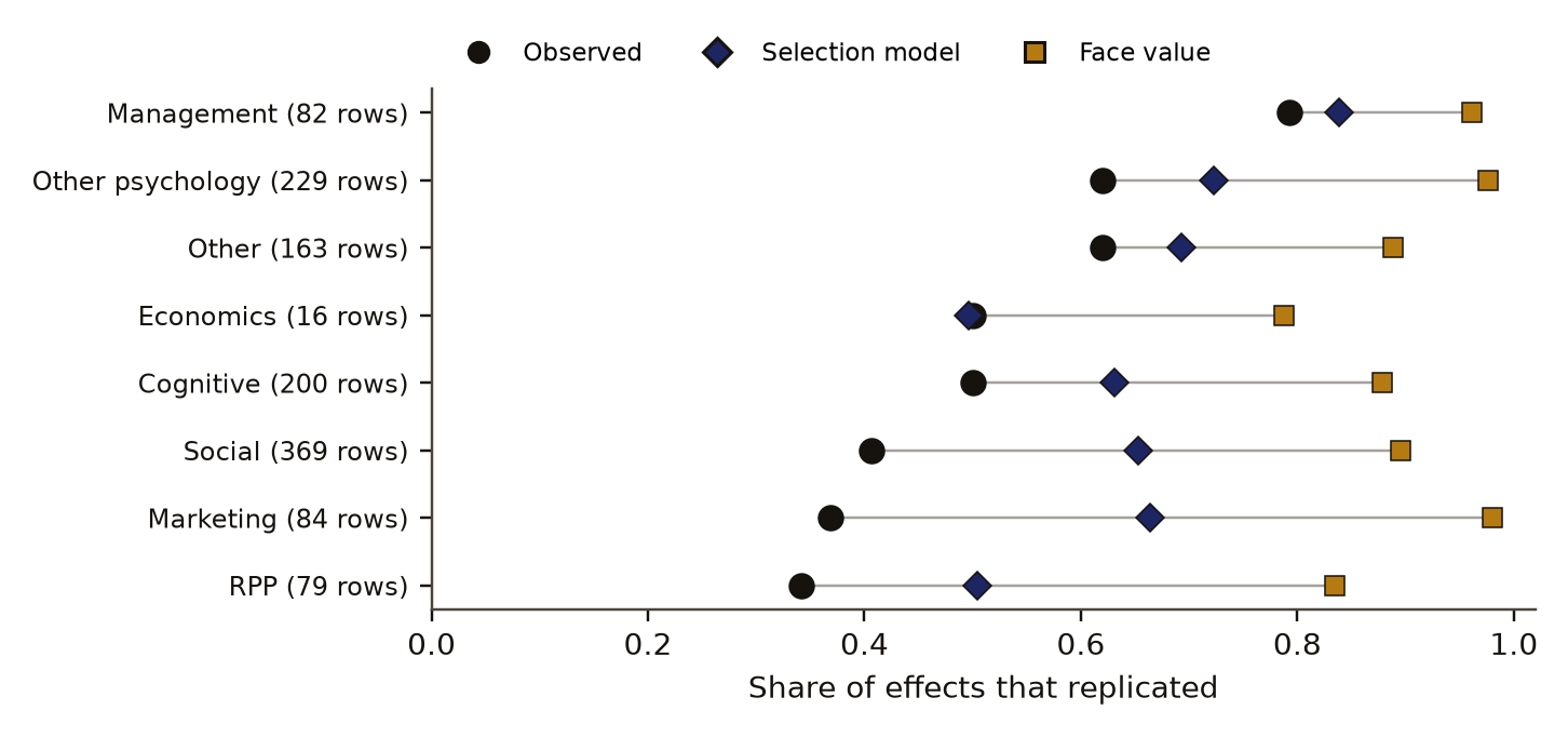
By field (Table 3, Figure 2), skill over the base rate was positive in three of the six fields the run counted as large (cognitive, marketing, other, other psychology, the Reproducibility Project and social; economics with 16 rows and management with 82 were left out), short of the preregistered target of 75 percent. The project counts by field sum to 342, more than the 307 clusters, because a cluster with rows in two fields is counted in each. The model's predicted rate sat above the observed rate in seven of the eight fields and below face value in all eight. For the Reproducibility Project the model predicted a success rate of 0.50 against 0.34 observed, where face value predicted 0.83; in social psychology it predicted 0.65 against 0.41, where face value predicted 0.89.
c4 observed, evidence for claim 4
- The numbers in claim 4
- 0.50; 0.34; 0.83; 0.65; 0.41; 0.89 matches the result file, 2026-11-09
- Chart 4
- Replication rate by held-out field: observed, the selection model's forecast, and face value.
- Chart 5
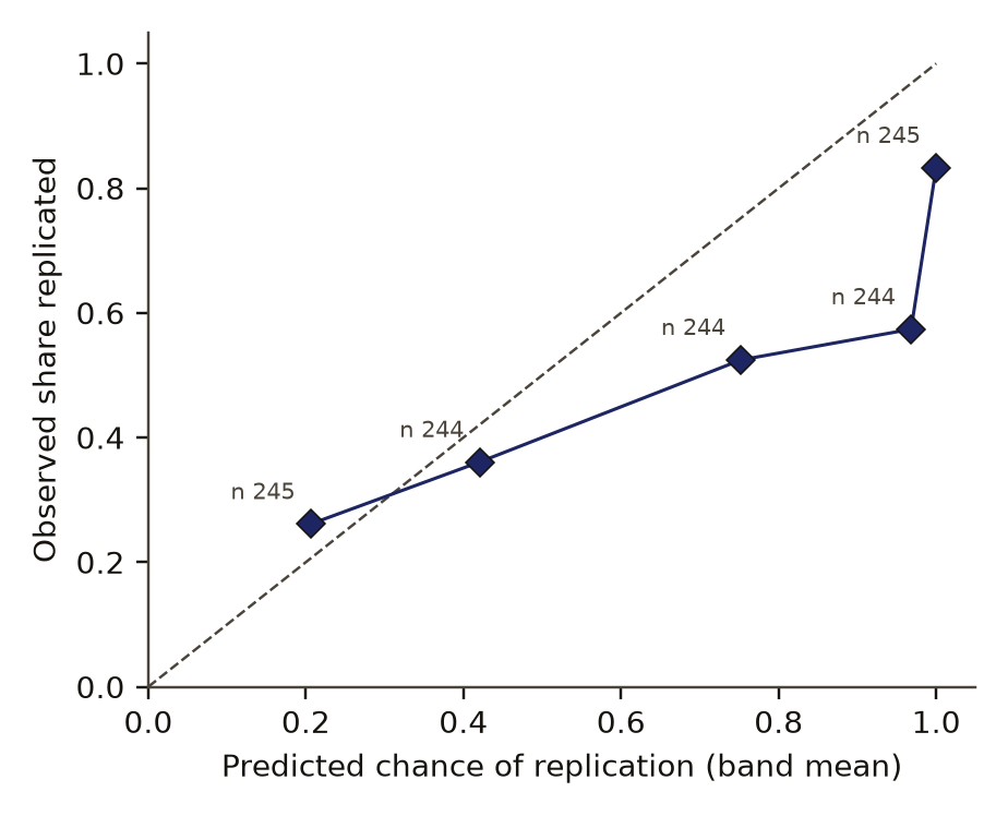
- Calibration of the selection model: the chance it gave against how often effects replicated.
- Basis
- observed: measured in this study, with a result file
share of effects that replicated
- selection model forecast
- face value forecast
- observed
Data behind chart 4 8 rows
| Field | Effects | Projects | Observed | Selection model | Face value | Skill over the base rate |
|---|---|---|---|---|---|---|
| Reproducibility Project | 79 | 79 | 0.34 | 0.50 | 0.83 | 0.048 |
| Social | 369 | 83 | 0.41 | 0.65 | 0.89 | −0.050 |
| Marketing | 84 | 6 | 0.37 | 0.66 | 0.98 | −0.053 |
| Cognitive | 200 | 50 | 0.50 | 0.63 | 0.88 | 0.020 |
| Economics | 16 | 7 | 0.50 | 0.50 | 0.79 | −0.006 |
| Other | 163 | 43 | 0.62 | 0.69 | 0.89 | −0.002 |
| Other psychology | 229 | 70 | 0.62 | 0.72 | 0.98 | 0.016 |
| Management | 82 | 4 | 0.79 | 0.84 | 0.96 | 0.088 |
Read from result.json, run 20261031T082124Z. SHA-256 of the run's file 8b1e7efec11d1d4a554de5e95028402756b0b5848cefe9cb014128686b4f2d1e and of the published copy 0c225e5cf3d1e641b3ef85b0272454a87559f43c272bce397a8e3a9ac61337ea. In the copy, file paths are cut to the file name and the layout (indentation, line endings) may differ; every value is the same.
share that replicated
mean forecast chance of replication
- selection model, one point per band
- perfect calibration
Data behind chart 5 5 rows
| Band | Effects | Mean forecast | Share that replicated |
|---|---|---|---|
| 1 | 245 | 0.206 | 0.261 |
| 2 | 244 | 0.420 | 0.361 |
| 3 | 244 | 0.752 | 0.525 |
| 4 | 244 | 0.968 | 0.574 |
| 5 | 245 | 1.000 | 0.833 |
Read from result.json, run 20261031T082124Z. SHA-256 of the run's file 8b1e7efec11d1d4a554de5e95028402756b0b5848cefe9cb014128686b4f2d1e and of the published copy 0c225e5cf3d1e641b3ef85b0272454a87559f43c272bce397a8e3a9ac61337ea. In the copy, file paths are cut to the file name and the layout (indentation, line endings) may differ; every value is the same.
The forecasts were also miscalibrated at the top, as Figure 3 shows. In five bands of equal count, calibrationDefinition: calibration forecast verification Agreement between forecast probabilities and observed frequencies: among effects given a chance near 0.7, about 70 percent should replicate. Checked here in five bands of equal count. Excludes discrimination, the separate question of whether higher forecasts go with more successes. full definition was close in the lowest two and overconfident above: effects given a mean chance of 0.97 replicated at 0.57, and effects given 1.00 replicated at 0.83.
The prior's shape did not hold up. The spike-and-normal prior beat a single normal by 192 in BIC (4,946.8 against 5,138.4), passing its rule of 10. A two-normal mixture beat the spike by 289 (4,657.5). On all originals the fitted was 0.82 and 0.51, and that description is a poor one. The transport variance hit the top of its grid, 1.0 on the Fisher z scale, in every fold.
On the 701 rows whose effect type carries a sign, the selection model scored 0.273, face value 0.402 and the base rate 0.256. The ranking of these three is the same as in the full set. With each project weighted equally, a preregistered sensitivity analysis with no decision rule attached, the selection model scored 0.244 against the base rate's 0.256 (Table 1), so the point comparison with the base rate changes sign when projects are weighted equally. No interval was computed for that version, and the preregistered verdict uses the row-weighted score.
Real skill over the base rate was -0.004, above the 95th percentiles of both shuffle controls (-0.110 and -0.092; p 0.002 and 0.005). Table 4 sets the forecasts written before the run against the outcomes.
Discussion
The result splits the selection reading in two. The part about level holds: forecasts that ignore the filter are badly overconfident, and modelling the filter brings the Brier score down from 0.402 to 0.260. This is the pattern Gelman and Carlin [5] describe, measured here as forecast error on held-out fields.
The part about picking effects fails. A forecast that ignores every effect's statistics and uses the training success rate does as well. On Brier score, the model's spread of forecasts across effects adds nothing over the base rate, and its top bands are overconfident. The logistic model, which uses the same original statistics without a model of selection, does better. A selection model with a rigid prior shape spends its freedom on the level and leaves the ranking to the prior, and the prior fits poorly by BIC.
The transport term points the same way. Allowing the replication's true effect to drift from the original's improved the score to 0.232, and its variance ran to the top of the grid in every fold. The gap between originals and replications on these data is larger than the selection model with a fixed true effect accounts for. Hidden moderators, differences in fidelity, real change over time and design differences ignored by the Fisher z standard error could all add to it, and the original statistics cannot tell them apart.
Limitations
- An earlier summary of ours said the model corrects the replication rate. Read against the table, it only shrinks the gap: the Reproducibility Project forecast missed by 0.16 against a preregistered tolerance of 0.05.
- The two-normal prior fitted better by BIC, so of 0.82 should not be read as a share of false hypotheses. The two-normal prior was compared by BIC only and was not tested on held-out fields.
- Fisher z standard errors ignore study design, so within-person studies look noisier than they are. Unsigned effect types assume the same direction in original and replication. Effects were converted from mixed metrics, and beta was treated as r.
- FReD has large nested projects; one has 156 rows. Management has 82 rows from 4 projects.
- Fields are our own coarse buckets.
- The Reproducibility Project forecast was not blind to its published rate, and the data's category counts were seen before the lock.
- The model predicts from original statistics. It cannot say why an effect failed, and a forecast on one effect is no verdict on that effect, its authors or their field.
- Scoring was done by our own code and was not blind.
Evidence
Mixed. The model beat taking originals at face value (the 95 percent interval of the Brier gain starts at 0.108). It did not beat the base rate (the interval starts at -0.039) and it lost to a small logistic model. Skill was positive in half the fields against a bar of three quarters, and its Reproducibility Project rate missed by 0.16 against a tolerance of 0.05. The preregistered kill rule fired, so the claim that the model picks which effects replicate is withdrawn.
Figures
These are the paper's own figures, numbered as in the PDF, and each "Figure" reference in the text points here. The charts on this page redraw the same results from the result files and carry their own numbers.
Tables
| Forecast | Brier | Project-weighted |
|---|---|---|
| Logistic regression | 0.223 | 0.231 |
| Selection model with transport term | 0.232 | 0.234 |
| Base rate | 0.256 | 0.256 |
| Selection model | 0.260 | 0.244 |
| Normal prior, no spike | 0.345 | 0.344 |
| Face value | 0.402 | 0.426 |
| Comparison | Difference | 95% interval | p | q |
|---|---|---|---|---|
| Face value | 0.142 | 0.108 to 0.186 | 0.00025 | 0.0005 |
| Base rate | -0.004 | -0.039 to 0.027 | 0.811 | 0.811 |
| Logistic regression | -0.037 | -0.069 to -0.011 | 0.010 | 0.014 |
| Normal prior, no spike | 0.085 | 0.059 to 0.118 | 0.00025 | 0.0005 |
| Field | Rows | Projects | Observed | Predicted | Face value | Skill |
|---|---|---|---|---|---|---|
| Cognitive | 200 | 50 | 0.50 | 0.63 | 0.88 | 0.020 |
| Economics | 16 | 7 | 0.50 | 0.50 | 0.79 | -0.006 |
| Management | 82 | 4 | 0.79 | 0.84 | 0.96 | 0.088 |
| Marketing | 84 | 6 | 0.37 | 0.66 | 0.98 | -0.053 |
| Other | 163 | 43 | 0.62 | 0.69 | 0.89 | -0.002 |
| Other psychology | 229 | 70 | 0.62 | 0.72 | 0.98 | 0.016 |
| Reproducibility Project | 79 | 79 | 0.34 | 0.50 | 0.83 | 0.048 |
| Social | 369 | 83 | 0.41 | 0.65 | 0.89 | -0.050 |
| Quantity | Forecast | Outcome |
|---|---|---|
| Brier, selection model | 0.21 | 0.260 |
| Brier, face value | 0.27 | 0.402 |
| Brier, base rate | 0.235 | 0.256 |
| Brier, logistic | 0.215 | 0.223 |
| Fitted pi0 and tau | 0.5 and 0.3 | 0.82 and 0.51 |
| Reproducibility Project predicted rate | 0.40 | 0.50 (observed 0.34) |
| Beats face value | probability 0.9 | yes |
| Beats base rate | probability 0.7 | no |
| Beats logistic | probability 0.3 | no |
| Spike beats normal by BIC 10 | probability 0.5 | yes |
| Share of fields with positive skill | 0.6 | 0.5 |
| Share at least 0.75 | probability 0.35 | no |
| Skill above shuffled-original control | probability 0.6 | yes |
Appendix A. The preregistered verdicts
Each verdict is a set of rules written before the run. A verdict passes only when every rule holds. Values are read from the run's result file.
| Verdict | Deciding rule | Value | Holds |
|---|---|---|---|
| Planted check | pi0 error below 0.1; rate error below 0.03; beats face value in at least 0.9 of datasets | 0.051; 0.009; 1.00 | yes |
| Data check | reported Reproducibility Project successes within 4 of 35; FReD label gap at least 0.3 | 1; 0.71 | yes |
| Beats face value | lower interval bound of the difference above 0 | 0.108 | yes |
| Beats base rate | lower bound above 0; skill above shuffled-outcome 95th percentile (-0.110) | -0.039; -0.004 | no |
| Originals add skill | skill above shuffled-original 95th percentile (-0.092) | -0.004 | yes |
| Beats logistic | lower interval bound of the difference above 0 | -0.069 | no |
| Spike needed | BIC of spike minus normal below -10 | -191.6 | yes |
| Most fields show skill | share of large fields with positive skill at least 0.75 | 0.5 | no |
| Reproducibility Project rate | forecast error at most 0.05 | 0.163 | no |
Numbers recorded in our publication register
| What | Value |
|---|---|
| Sample | 1222 effects, 307 project clusters |
| Main estimate and interval | project-cluster bootstrap 95 percent |
| Forecast against outcome | beating the base rate was given a probability of 0.7; it failed at -0.004 |
| Known-answer check | planted mixtures; 34 reported Reproducibility Project successes in the rows kept, against the 35 published |
As recorded in the publication register, the summary row each finding gets; the paper's own numbers above were re-read from the result files.
What lowers it
- blinding Not blind. The Reproducibility Project forecast was not blind to the published 36 percent. from our publication register, on blinding
- scoring Graded by the same agent that ran it. from our publication register, on who scored it
- depth of reading The cited literature was read at the level of abstracts, publisher pages and search summaries; full texts were not read. from the Verified section
What holds it up
- preregistration Preregistered and hash-locked before the run (sha256 93132f99). from the Reproduce section
- control Controls: shuffled outcomes, shuffled originals, planted truths, data checks. from our publication register, on controls
- open data Public data. from our publication register, on the data licence
Where the claim stands
- lead
- hypothesis
- thesis
- conjecture
- theorem
- law candidate
- killed
A preregistration with pass-or-fail rules is on file, which this rung needs. The next rung needs a named rival reading beaten by a decisive observation, and none is on file. Tier B: A real held-out result on public data, with its planted and data checks passing. Related methods exist; a search on 9 November 2026 found no test of this exact design, which does not show that none exists. Conversions between effect measures still need review.
Trail
Versions
- v3 2026-11-14, this page corrected, 1 item; the PDF and its BuildTeX source are still paper version 1.0
- v2 2026-11-09, paper version 1.0, first published PDF sha256 eeb1c60eee68fe44
- v1 2026-10-31, entered in the findings ledger
Corrections
2026-11-14 number found by a review of the published pages
A review of the published page found the outcome word at odds with the page. now The header said held while the preregistered kill rule had fired and four of nine verdicts had failed; it now says mixed, and the header shows the verdict count. The results now name the six fields the run counted as large and say why the project counts by field sum to more than the 307 clusters. The register line that read 35 Reproducibility Project successes now gives the 34 the kept rows carry, against the 35 published.
2026-10-31 scope found by the study itself, before publication
The original heading and kill line in our findings ledgerDefinition: findings ledger our records The append-only, dated list of every result we have recorded, numbered F1, F2 and on. Corrections are added as new dated lines and old entries are never rewritten. Excludes a curated list of successes. full definition said the model corrects the rate. now Read against the table it only shrinks the overstatement. This paper states the narrower reading throughout.
Standing, and the ledger entries it rests on
2026-10-31 extended F270
Set by hand from findings ledger entry F270, dated 2026-10-31: the same replication records. Rests on findings ledger, F270.
Each correction is a dated note; the findings ledger is never rewritten, and a note governs where it differs.
Ledger and version dates up to publication are local dates in US Pacific time. Clock times in the text are UTC, seven or eight hours ahead, so a lock or a run stamped just after midnight UTC belongs to the previous local day. Corrections from 14 November 2026 on are dated in UTC.
References
- Open Science Collaboration (2015). Estimating the reproducibility of psychological science. Science 349(6251), aac4716. doi:10.1126/science.aac4716 run here Licence: RPP CC0, FReD CC BY 4.0 used in Introduction, Data and provenance
- Open Science Collaboration. Reproducibility Project: Psychology, data files. Open Science Framework project ezcuj. CC0. Read 31 October 2026. run here Licence: RPP CC0, FReD CC BY 4.0 used in Data and provenance
- FORRT Replication Database (FReD). Open Science Framework, doi:10.17605/OSF.IO/9r62x. CC BY 4.0. Read 31 October 2026. run here Licence: RPP CC0, FReD CC BY 4.0 used in Data and provenance
- Röseler, L., Kaiser, L., Doetsch, C. and others. The Replication Database: documenting the replicability of psychological science. Open access at PubMed Central, PMC12270267. abstract or summary, 2026-11-09: abstracts, publisher pages and search summaries; full text not read used in Introduction
- Gelman, A. and Carlin, J. (2014). Beyond power calculations: assessing Type S (sign) and Type M (magnitude) errors. Perspectives on Psychological Science 9(6), 641-651. doi:10.1177/1745691614551642 abstract or summary, 2026-11-09: abstracts, publisher pages and search summaries; full text not read used in Introduction, Discussion
- Bartos, F. and Schimmack, U. (2022). Z-curve 2.0: estimating replication rates and discovery rates. Meta-Psychology 6, MP.2021.2720. abstract or summary, 2026-11-09: abstracts, publisher pages and search summaries; full text not read used in Introduction, Discussion
- Altmejd, A., Dreber, A., Forsell, E., Huber, J., Imai, T., Johannesson, M., Kirchler, M., Nave, G. and Camerer, C. (2019). Predicting the replicability of social science lab experiments. PLoS ONE 14(12), e0225826. doi:10.1371/journal.pone.0225826 abstract or summary, 2026-11-09: abstracts, publisher pages and search summaries; full text not read used in Introduction, Discussion
Cited by later findings
- F270 extended, the same replication records, 2026-10-31 (record findings ledger, F270). A single split of noise and field bias ranks failed replications on the same RPP and FReD set (Brier 0.222 against 0.256), adding nothing to the z value alone.
Reproduce
Data
- Open Science Collaboration (2015). Licence: RPP CC0, FReD CC BY 4.0. https://doi.org/10.1126/science.aac4716
- Open Science Collaboration. Licence: RPP CC0, FReD CC BY 4.0.
- FORRT Replication Database (FReD). Licence: RPP CC0, FReD CC BY 4.0. https://doi.org/10.17605/OSF.IO/9r62x
Preregistration
sha256 93132f995daad75ca338b5ac8442d262da99b52b5c59d7f1dbfa83fcba3a466f
plan 1a6cc22eb03f2b7a168e32ecd696a312affde7a8b1da74809a97434e3f9c7b33
Steps
- Data: download the Reproducibility Project Psychology data and FReD from the Open Science Framework, and remove the Reproducibility Project rows from FReD.
- Convert effects to Fisher z with eqs. 1 and 2, and keep originals with above 1.96 in absolute value.
- Fit the prior of eq. 3 by the selection likelihood of eq. 4 on seven fields, forecast the eighth with eq. 5, and repeat for every field.
- Score with eq. 6; compare forecasts with a 2,000-draw project bootstrap and 4,000 project sign flips, adjusted by Benjamini-Hochberg.
- Preregistration SHA-256: 93132f995daad75ca338b5ac8442d262da99b52b5c59d7f1dbfa83fcba3a466f. Plan SHA-256: 1a6cc22eb03f2b7a168e32ecd696a312affde7a8b1da74809a97434e3f9c7b33. Run 20261031T082124Z.
Cost. The analysis took 13 seconds and both controls under one second on one desktop computer, as timed in the result file. The study was not re-run for this paper.
Downloads
- Whitepaper, PDF F172.pdf, 601 KB
- BuildTeX source F172.bld, 37 KB
- Build receipt F172.buildtex.json, 1 KB
- BuildLang doc module doc.bld, 5 KB, imported by the source
The PDF is typeset by BuildTeX from F172.bld, which is written from the same source as this page. The receipt records the source's SHA-256 and the PDF's (eeb1c60eee68), so anyone can rebuild it and compare. The copy here has its hidden author field blanked, as the site does for every file it publishes; blank the same field in a rebuild before comparing. The name stays on the first page.
Verified
Verified on 2026-11-09. On 9 November 2026 the row, project and conversion counts, the six Brier scores and their project-weighted versions, the four comparison differences with intervals, p and q values, the per-field rows, projects, rates and skills, the five calibration bands, the planted and data-check values, the BIC values, the fitted prior and transport values, the signed-row sensitivity, both shuffle quantiles and all nine verdicts were re-read from the run's result file. They match the findings ledger. The forecasts were read from the preregistration. The preregistration's SHA-256 was recomputed on that date and matches the hash in the result file. All three figures were drawn by a script that reads only that result file.
Not checked. The study was not re-run for this paper. The literature in the introduction was found by searches run on 9 November 2026 and read at the level of abstracts, publisher pages and search summaries; the full texts were not read. A Verified lineDefinition: Verified line our publication rule The closing statement of what was checked for publication, by what means, with what result and on what date. Anything not checked is named as such. Excludes a claim that the finding is true. full definition lists what was checked, and anything not listed was not checked.
Terms on this page
Each term is defined where it is first used on this page. Each name below opens its entry in the findings glossary, which lists every page that uses it.
- significance filter (winner's curse) metascience and statistics first use
- selection model meta-analysis and statistics first use
- preregistration research method (metascience) first use
- planted check research method; called a positive control in experimental science first use
- control statistics and experimental design first use
- kill condition research method (our usage, after Popper's falsification) first use
- verdict research method (our usage) first use
- void research method (our usage) first use
- Fisher z statistics first use
- face-value forecast forecasting, our usage first use
- base-rate forecast forecasting first use
- logistic regression statistics first use
- Brier score forecast verification first use
- leave-one-field-out test statistics, cross-validation first use
- 95% interval statistics first use
- project-cluster bootstrap statistics first use
- sign-flip permutation test statistics first use
- Benjamini-Hochberg correction statistics, multiple testing first use
- BIC statistics, model comparison first use
- null distribution statistics first use
- calibration forecast verification first use
- findings ledger our records first use
- Verified line our publication rule first use
To report an error, name the finding, the claim number and the source on the Work page, which gives the address. Accepted corrections join the Trail with their date.