
Findings F166 Psychology and perception, Society and economics, Method and statistics found 2026-10-31
Our combined value formula lost to plain prospect theory on 11,759 risky choice problems
We tested our own formula for how people value risky options, prospect theory plus terms for information, threat and drive, against a richer version of prospect theory on the public choices13k data. It never beat that richer model by the margin we set in advance (with feedback it led by 0.001 against a bar of 0.005), so we retired it. Fitted loss aversion came out at 1.16 when people chose from descriptions and 0.89 when they learned from feedback.
- Tier
- D, honest null
- Outcome
- prediction failed
- Rung
- killed
- Verdicts
- 4 passed, 3 failed
- Kill rule
- fired
- Corrections
- 3, latest 2026-11-14
- Version
- v3, 2026-11-14
- Redo it
- Reproduce
Download PDF 556 KB BuildTeX source F166.bld
What this means for a reader
Adding terms to a model of choice will almost always improve its fit a little. The fair test is whether the new terms beat a version of the old theory given a similar number of extra parameters, three against our four. Ours did not, so the terms we named after information, threat and drive describe where prospect theory misfits, and they do not add a new account of why people choose. The loss aversion we measured sits near 1, well below the classic 2.25, which says this number depends on the task that measures it.
Objection
Entropy, loss probability and the mean and mean square of outcomes are one reading of information, threat and drive. Another reading could score differently, so the result covers this operationalisation only.
What would change the call. Person-level data and a preregistered reading of information gain.
From the paper's first stated limitation; our register records no separate objection.
Abstract
We had written a single value formula for risky choice: prospect value plus a term for the information a gamble resolves, a term for the threat of a loss, and a term for drive toward a setpoint. We tested it on the public choices13k data, 1,928 problems answered without outcome feedback and 9,831 answered with it, against cumulative prospect theory and against a flexible prospect theory with comparable room to absorb misfit (three extra parameters against our four). The kill rule was fixed before any real fit. The combined formula never beat the flexible prospect theory by the preregistered margin: cross-validated R² 0.634 against 0.645 without feedback and 0.597 against 0.596 with it, against a bar of 0.005. Without feedback, the joint gain of the four added terms, 7.6 in deviance, sat below the 95th percentile of both null controls, 52.0 and 58.9. With feedback two of the terms help as corrections to prospect theory, and the drive term does not. The kill rule fired, and the formula is retired as a model of risky choice. Fitted loss aversion was 1.16 (1.05 to 1.30) without feedback and 0.89 (0.86 to 0.93) with feedback.
c1 observed, evidence for claim 1
- The numbers in claim 1
- 0.634; 0.645; 0.597; 0.596; 0.005 matches the result file, 2026-11-09
- Chart 1
- How the test was built: five models, one planted check and two null controls.
- Chart 2
- Every rule fixed in advance, the value it tested and the bar it had to clear.
- Chart 3
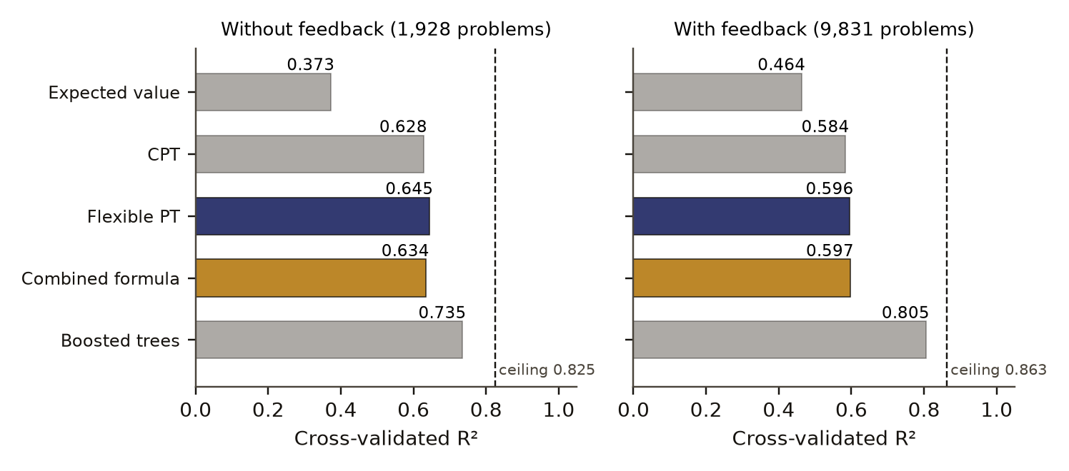
- Held-out fit of each model, without and with feedback.
- Basis
- observed: measured in this study, with a result file
c2 observed, evidence for claim 2
- The numbers in claim 2
- 7.6; 95; 52.0; 58.9 matches the result file, 2026-11-09
- Chart 4
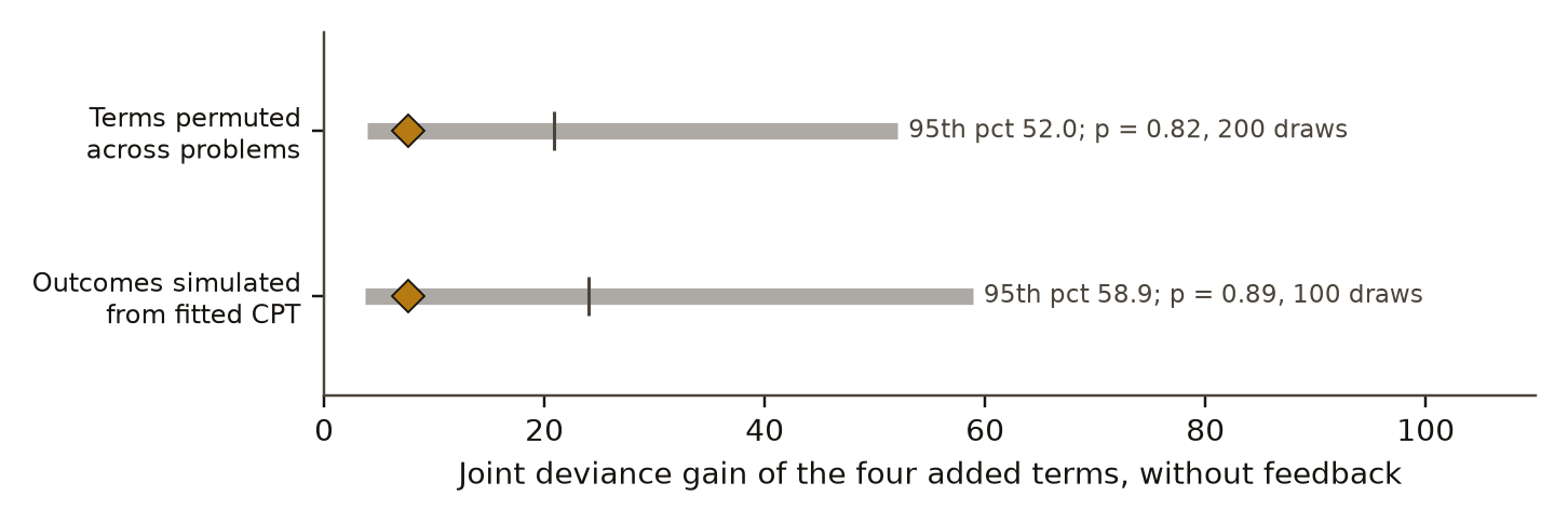
- Without feedback: the joint gain of the four added terms against two null controls.
- Basis
- observed: measured in this study, with a result file
c4 observed, evidence for claim 4
- The numbers in claim 4
- 1.16; 1.05; 1.30; 0.89; 0.86; 0.93 matches the result file, 2026-11-09
- Chart 5
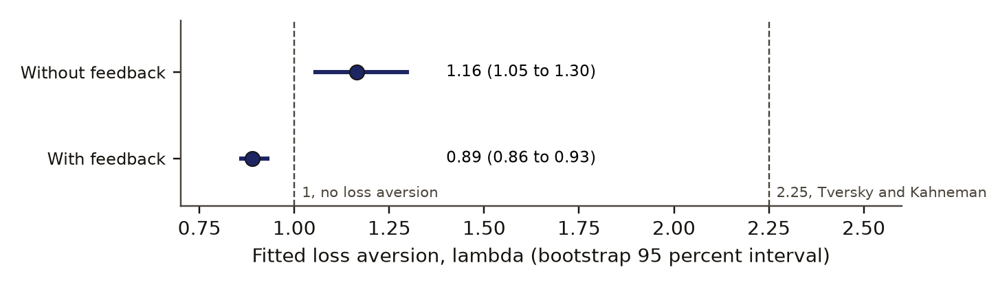
- Fitted loss aversion in each setting.
- Basis
- observed: measured in this study, with a result file
Introduction
Cumulative prospect theoryDefinition: cumulative prospect theory (CPT) behavioural economics A model of choice between gambles with a value function concave for gains and steeper for losses, a loss aversion coefficient and a probability weighting function applied to cumulative probabilities. Here six parameters. Excludes any account of the feelings or brain processes behind a choice. full definition [2] describes a choice between gambles with three ingredients: a value function that is concave for gains and steeper for losses, a loss aversionDefinition: loss aversion behavioural economics The factor lambda by which a loss weighs more than an equal gain in the value function. 1 means losses and gains count alike. Excludes a dislike of risk as such, which curvature and weighting carry. full definition coefficient that scales losses, and a weighting functionDefinition: probability weighting function behavioural economics A function that maps a stated probability to the weight a choice gives it, so that small chances can count for more than their size and large ones for less. Excludes a person's belief about the odds, which in these problems are stated. full definition that bends probabilities. The theory comes from behavioural economics and describes choices; it gives no account of the feelings behind them. Loss aversion is the factor by which a loss weighs more than an equal gain, so 1 means losses and gains count alike, and it says nothing about a dislike of risk as such. The weighting function maps a stated probability to the weight a choice gives it, so small chances can count for more than their size; it is no belief about the odds. Tversky and Kahneman reported a median of 2.25 from their own experiment. Brown, Imai, Vieider and Camerer [3] collected 607 estimates of from 150 articles published from 1992 to 2017 and pooled them in a meta-analysisDefinition: meta-analysis statistics, research synthesis The statistical pooling of published estimates of one quantity into a summary and a measure of their spread. Excludes collecting new data. full definition, the statistical pooling of published estimates of one quantity, which collects no new data of its own.
Peterson, Bourgin, Agrawal, Reichman and Griffiths [1] ran the largest risky choice experiment to that date, choices13k, with choice rates on 13,006 problems collected online. They used it to compare classical decision theories with machine-learning models and to search for better theories. Thomas and colleagues [6] argued that the choice behaviour in choices13k contains structured decision noise when compared with a laboratory data set, which bears on how much of the gap between theories and flexible learners is psychology.
The data set also separates problems answered with and without feedback on outcomes. Hertwig, Barron, Weber and Erev [5] reported that people choose as if they overweight rare events when choosing from descriptions and underweight them when choosing from experience, the pattern later called the description-experience gapDefinition: description-experience gap decision research The pattern that people choose as if they overweight rare events when choosing from stated odds and underweight them when they learn the odds from sampled outcomes. Excludes differences in the gambles themselves. full definition. In decision research the term means that difference between choices from stated odds and choices learned from sampled outcomes; it excludes any difference in the gambles themselves. We analysed the two settings apart for that reason.
Our own starting point was a combined value formulaDefinition: combined value formula (COMB) our usage CPT's value difference plus four added terms in one choice rule: entropy for information, loss probability for threat, and the mean and mean square of outcomes for drive toward a setpoint. Ten parameters. Excludes any claim about mechanisms in the brain, and any reading of the terms other than this operationalisation. full definition from earlier notes in this project, a name of ours for prospect value plus four added terms in one choice rule, standing for three ideas: information, threat and drive, which makes no claim about mechanisms in the brain. It adds to prospect value a term for the information a gamble resolves, a term for the threat of a loss, and a term for reduction of a drive toward a setpoint. This paper is a test of that formula, and the formula is ours to retire.
Preregistration and design
The design was written and hash-locked on 31 October 2026 at 08:02 UTC as a preregistrationDefinition: preregistration research method (metascience) A dated written plan for a study, fixed and hash-locked before any result is seen: the question, the data, the statistic, the controls, the forecasts and the kill conditions. Excludes a plan revised after looking at the outcome, and a protocol written only for the record after the run. full definition, a practice from clinical trials and psychology: a dated plan fixed before any result is seen, so a plan revised after a look at the outcome does not qualify. Before writing it we had seen the file schemas, the row counts and outcomes simulated by the study code. No real outcome had been fitted.
- data1,928 and 9,831 problemschoices13k, split by whether people saw feedback after each choice.
- measurementFit five models, score held-out R²Expected value, cumulative prospect theory, a flexible prospect theory, the combined formula and boosted trees.
- planted checkPlanted model picked in 6 of 6Data simulated from a known model. Model selection had to pick that model in more than 80 percent of sets.
- controlControl 1: terms permutedThe added terms shuffled across problems, 200 times.
- controlControl 2: outcomes simulatedChoice rates drawn from the fitted prospect theory, 100 times.
- rule set in advanceRule: R² gain of at least 0.005Over flexible prospect theory, with a BIC gain of more than 10. Fixed before the run.
- failedCombined formula beats flexible prospect theoryGain −0.011 without feedback and 0.0009 with it.
Read from result.json, run 20261031T080226Z. SHA-256 of the run's file 6b6a2c429eabe63effb8a055cb975e337c929e517d9e7ecb695d35292d836a92 and of the published copy ff1e84e6f4b6c8cd45a3ac469339cc2e7848d24bf98471a51ef1143a4da0a326. In the copy, file paths are cut to the file name and the layout (indentation, line endings) may differ; every value is the same.
The locked file names the data, the two settings, every model, the scoring, the planted checksDefinition: planted check research method; called a positive control in experimental science Data built so that the right answer is known, run through the same analysis before the real data, to show that the analysis can see the effect when it is there. Excludes any check made on the real data, which cannot show what the analysis misses. full definition, both controlsDefinition: control statistics and experimental design A version of the data with the structure under test removed (for example shuffled or pooled), scored the same way as the real data, so the real score has something to beat. Excludes a comparison with a different dataset or with a published number. full definition, the forecasts and the kill ruleDefinition: kill condition research method (our usage, after Popper's falsification) A rule written in the preregistration that, when met, decides against the claim with no room for judgement after the run. Excludes reasons found after the run for setting a result aside. full definition. A planted check runs data with a known answer through the same analysis first, to show the analysis can find an effect when it is there, which no check on real data can show. A control is a version of the data with the structure under test removed, scored the same way as the real data; a published number from another study is no control. The kill rule decides against the claim when it is met, with no room for judgement after the run. The question it states is whether the combined formula predicts human risky choice better than cumulative prospect theory, and better than a richer pure prospect theory that could absorb the same misfit. Nothing was added after the run. The preregistration's SHA-256 is given in the reproduction section.
Kill and void conditions, as written:
- If the combined formula fails to beat the flexible prospect theory in both settings by 0.005 in cross-validated R² with a quasi-binomial BIC change below -10, the formula is retired as a model of risky choice, and its added terms are read as patches for prospect theory misfit whatever their permutation p values say.
- If the planted check fails, every other verdictDefinition: verdict research method (our usage) The pass or fail of one preregistered rule set against the run's numbers, read off by code. Excludes an interpretation written after reading the numbers. full definition is voidDefinition: void research method (our usage) The verdict of a run whose planted check failed or whose sample fell below its stated minimum. It says nothing for or against the claim. Excludes a null result, which comes from a working instrument. full definition. A verdict, in our usage, is the pass or fail of one preregistered rule set read off by code. A void verdict says nothing for or against the claim, unlike a null result from an instrument that works.
Data and provenance
The data are choices13k [1], the selections table and the problems file from the authors' public repository. Each row gives, for one problem, the share of participants who chose option B over option A, the number of participants and the between-person standard deviation of that share. There is no person-level input.
We kept rows marked unambiguous and split them by the feedback flag: 1,928 problems answered without outcome feedback, which we call the description settingDefinition: description setting our usage, after decision research The 1,928 choices13k problems answered without outcome feedback, where people chose from stated odds alone. Excludes the 9,831 problems answered with feedback on outcomes. full definition because people chose from stated odds alone and learned no outcomes along the way, and 9,831 answered with feedback. In each setting each problem appears once. The repository states no licence. We used a local research copy and report only statistics computed from it.
A join check ran before the lock. The problems file uses row positions in the selections table as its keys, and problem identifiers do not match them. On a dry run with simulated outcomes the join by identifier matched 0.015 of rows; after the fix the match was 1.0 in both settings, checked by recomputing each problem's expected value from both files.
Methods
The choice rule
Every value model predicts the log oddsDefinition: log odds statistics For a rate p, the natural log of p divided by 1 minus p. 0 at an even split and unbounded toward certainty. Excludes any information beyond the rate, of which it is a rescaling. full definition of choosing B from the difference in value between the options. The log odds of a rate is , a statistics rescaling that is 0 at an even split and adds no information to the rate:
where is the predicted rate, an intercept and a sensitivity. Models were fitted by binomial likelihoodDefinition: binomial likelihood statistics Fitting by choosing the parameters under which the observed counts of B choices are most probable, treating each choice as an independent draw at the predicted rate. Here five choices per listed participant. Excludes extra scatter between problems, which the dispersion handles. full definition on the observed rates, the statistics method that picks the parameters under which the observed counts of B choices are most probable, treating each choice as an independent coin with the predicted rate, counting five choices per listed participant, the count the study code uses for each problem.
The models
The expected valueDefinition: expected value (EV) probability theory The probability-weighted average payoff of a gamble, used here as the baseline value model. Excludes any allowance for risk, loss or probability weighting. full definition baseline (EV), the probability-weighted average payoff from probability theory with no allowance for risk or loss, uses for outcomes with probabilities . Cumulative prospect theory (CPT) uses rank-dependent weightsDefinition: rank-dependent weights decision theory Decision weights that depend on where an outcome ranks among a gamble's outcomes, taken as differences of the weighting function at cumulative probabilities. Excludes weighting each outcome's probability on its own, as the original 1979 prospect theory did. full definition , decision weights that depend on where an outcome ranks among the gamble's outcomes and are taken as differences of the weighting function at cumulative probabilities, which excludes weighting each probability on its own, and a value function that for gains is
and for losses is , with . The weights come from the Tversky and Kahneman weighting function applied to cumulative probabilities, with its own for gains and for losses:
CPT has six parameters. The flexible prospect theory (FLEX) has separate curvature for gains and losses, , and the two-parameter Prelec weighting functionDefinition: Prelec weighting function decision theory A two-parameter probability weighting function, exp of minus delta times minus log p to the power gamma, that sets the curvature and the crossing point of the curve separately. Excludes the one-parameter Tversky and Kahneman function used in CPT. full definition [4] on each side, nine parameters in all. Prelec's function, from decision theory, sets the curvature and the crossing point of the weighting curve separately, a shape the one-parameter function cannot take:
The combined formula
The combined formula (COMB) keeps CPT and adds four terms to the log odds of eq. 1, each the value for option B minus the value for option A:
Here is the Shannon entropyDefinition: Shannon entropy information theory Minus the sum of p log2 p over a gamble's outcomes, in bits: how uncertain the outcome is before it happens, 0 for a sure thing. Excludes the sizes of the payoffs. full definition of the outcome distribution in bits, read as the information gained when the gamble resolves. In information theory entropy measures how uncertain an outcome is before it happens, 0 for a sure thing; it ignores the sizes of the payoffs:
is the probability of a loss, read as threat. is the mean outcome and the mean squared outcome. Those two carry the drive term: for a setpoint , the drive reductionDefinition: drive reduction motivation psychology, our operationalisation For a setpoint S, the quantity S squared minus (S minus x) squared for an outcome x, whose expectation is linear in the mean and mean square of outcomes. Excludes any measured need or state of the people choosing. full definition of an outcome is
so its expectation is linear in and . Drive reduction is a term from motivation psychology, here only the quadratic form above, and it excludes any measured need or state of the people choosing. The mean was divided by 10 and the mean square by 1,000 before fitting. COMB has ten parameters. Three reduced models add each term alone: CPT+H (entropy), CPT+T (loss probability) and CPT+D (mean and mean square).
Scoring
Each model was scored by 10-fold cross-validated R²Definition: cross-validated R² statistics and machine learning One minus the squared error of out-of-fold predictions over the variance of the observed rates, with 10 folds grouped by problem: the share of variance that predictions made without seeing those rates account for. Excludes in-sample R², which rewards fitting noise. full definition on the rates, with folds grouped by problem. Cross-validated R², from statistics and machine learning, is the share of variance in the observed rates that predictions made without seeing those rates account for, so it does not reward fitting noise as in-sample R² does. With out-of-fold predictions , observed rates and their mean ,
Each model was also scored by a quasi-binomial BICDefinition: quasi-binomial BIC statistics, model selection The Bayesian information criterion with the log-likelihood divided by the dispersion: a score that trades fit against the number of parameters, lower being better. Excludes an absolute test of a model, since it only compares models on the same data. full definition, with the dispersionDefinition: dispersion statistics, quasi-likelihood The factor phi by which observed rates scatter more than independent binomial choices would allow, taken from the COMB fit in each setting. Excludes a parameter of choice behaviour. full definition taken from the COMB fit in each setting (5.70 without feedback, 7.58 with it):
where is the binomial likelihood, the number of parameters and the number of problems. The Bayesian information criterion, a statistics score, trades fit against the number of parameters, lower being better; it compares models on the same data and gives no absolute test. The dispersion scales the likelihood for rates that scatter more than independent choices would allow, the quasi-binomial adjustment, and it is no parameter of choice.
Two references bound the value models. Gradient-boosted treesDefinition: gradient-boosted trees machine learning A predictor built by adding many small decision trees, each fitted to what the previous ones missed. Here a flexible learner's score on the same folds. Excludes a theory of choice, since it states no value function. full definition, fitted to the raw problem parameters and the four added terms with the same folds, give a flexible learner's score. The method, from machine learning, adds many small decision trees each fitted to what the previous ones missed; it predicts well and states no theory of choice. A sampling ceilingDefinition: sampling ceiling our usage, after reliability analysis One minus the mean sampling variance of the observed rates over their variance across problems: the share of variance not explained by finite samples of participants. Excludes noise of other kinds, such as the structured decision noise reported for these data. full definition, our bound, is the share of variance across problems not explained by sampling noise, . Here is the mean over problems of the squared between-person standard deviation divided by the number of participants, and is the variance of the observed rates.
Tests on the added terms
Each added term was tested with the fitted CPT log odds held as a fixed offsetDefinition: offset regression A part of the prediction fixed in advance and never refitted. Here the fitted CPT log odds, so an added term can only explain what CPT leaves over. Excludes refitting CPT together with the added term. full definition: the term was standardised, fitted by iteratively reweighted least squaresDefinition: iteratively reweighted least squares statistics, generalised linear models The standard routine for fitting a logistic model by repeated weighted least-squares steps. Excludes any effect on what is tested, since it is only the fitting method. full definition, and its devianceDefinition: deviance statistics, generalised linear models Twice the log-likelihood shortfall of a model against a perfect fit. A deviance gain is the fall in deviance when a term is added. Excludes any penalty for the added parameter. full definition gain was compared with 200 fits on the same term permuted across problems. An offset, in regression, is a part of the prediction fixed in advance and never refitted, so the term can only explain what CPT leaves over. Iteratively reweighted least squares is the standard fitting routine for such models, a means of fitting with no effect on what is tested. Deviance is twice the log-likelihood shortfall of a model against a perfect fit, so a deviance gain is the improvement in fit from the term, before any penalty for its parameter. The p valueDefinition: p value (from draws) statistics The share of control draws scoring at or above the real score, with one added to the count and to the number of draws, so it is never zero. Excludes a p value from a textbook formula that assumes a distribution. full definition is a p value from draws, as in permutation statistics, and assumes no textbook distribution; it counts one added to the numerator and the denominator:
where is the number of permuted gains at or above the real one and the number of permutations. The smallest possible value at 200 permutations is 0.005. The six p values, three terms in two settings, were corrected by Benjamini and Hochberg's procedureDefinition: Benjamini-Hochberg correction statistics, multiple testing A rule that adjusts a set of p values into q values so that, among the tests called significant, the expected share of false calls stays at or below a chosen rate q, here 0.05. Excludes the stricter Bonferroni rule, which bounds the chance of any false call. full definition at q 0.05. That multiple-testing rule keeps the expected share of false calls among the tests called significant at or below q, which is looser than the Bonferroni bound on any false call; the corrected values are q values.
The loss aversion intervalDefinition: 95% interval statistics The range that holds the middle 95 percent of the bootstrap or control draws for a number. We report it beside the number. Excludes a statement that the true value lies inside with 95 percent probability. full definition comes from refitting CPT on problems resampled with replacement: 100 resamples without feedback and 30 with feedback, with the 2.5th and 97.5th percentiles reported. This is a bootstrapDefinition: bootstrap statistics Refitting a model many times on problems resampled with replacement to read how much an estimate varies. Excludes an interval from a textbook formula that assumes a distribution. full definition, the statistics method that reads a number's spread from resampled data with no distribution assumed, and the interval holds the middle 95 percent of the resamples; it is no statement that the true value lies inside with 95 percent probability.
Controls and planted checks
The planted check ran on the description problems with their real participant counts. Three data sets were simulated from CPT with 1.6, and three from CPT plus an entropy term with coefficient 0.25, each with extra-binomial noiseDefinition: extra-binomial noise statistics Scatter in a choice rate from problem to problem beyond what independent choices would give, simulated here with a Beta distribution. Excludes a bias in the rate. full definition drawn from a Beta distribution. That is scatter in the choice rate from problem to problem beyond what independent coin flips would give, the kind of spread real aggregate rates show, and it adds no bias to the rate. Selection between CPT and COMB was by the quasi-binomial BIC. The rule required the right model in at least 5 of 6 data sets and recovered within 0.3 in at least 2 of 3. Model selection picked the true model in 6 of 6 planted data sets and recovered loss aversion within 0.3 in 3 of 3. The three recovered values were 1.64, 1.55 and 1.59. The check passed, and no verdict was voided.
c5 observed, evidence for claim 5
- The numbers in claim 5
- 6; 0.3; 3 matches the result file, 2026-11-09
- Chart 1
- How the test was built: five models, one planted check and two null controls.
- Chart 2
- Every rule fixed in advance, the value it tested and the bar it had to clear.
- Basis
- observed: measured in this study, with a result file
| Rule set in advance | Value | Bar | Result |
|---|---|---|---|
| Planted check: share of planted models picked, above 0.8 | 1.000 | 0.800 | held |
| Planted check: share of planted loss aversion recovered, above 0.6 | 1.000 | 0.600 | held |
| Join check: share of problems matched between files, above 0.999 | 1.000 | 0.999 | held |
| No feedback, against prospect theory: R² gain at least 0.005 | 0.0057 | 0.0050 | held |
| No feedback, against prospect theory: BIC change below −10 | −9.622 | −10 | failed |
| No feedback: smallest corrected p of a single term below 0.05 | 0.766 | 0.050 | failed |
| No feedback: joint gain above the permuted-terms 95th percentile | 7.623 | 52.042 | failed |
| No feedback: joint gain above the simulated-outcomes 95th percentile | 7.623 | 58.870 | failed |
| No feedback, against flexible prospect theory: R² gain at least 0.005 | −0.011 | 0.0050 | failed |
| No feedback, against flexible prospect theory: BIC change below −10 | 58.657 | −10 | failed |
| Feedback, against prospect theory: R² gain at least 0.005 | 0.013 | 0.0050 | held |
| Feedback, against prospect theory: BIC change below −10 | −304.361 | −10 | held |
| Feedback: smallest corrected p of a single term below 0.05 | 0.015 | 0.050 | held |
| Feedback, against flexible prospect theory: R² gain at least 0.005 | 0.0009 | 0.0050 | failed |
| Feedback, against flexible prospect theory: BIC change below −10 | −38.361 | −10 | held |
| No feedback: loss aversion interval above 1 | 1.055 | 1 | held |
| No feedback: loss aversion interval below 2.25 | 1.297 | 2.250 | held |
Data behind chart 2 17 rows
| Rule set in advance | Value | Bar | Result |
|---|---|---|---|
| Planted check: share of planted models picked, above 0.8 | 1.000 | 0.800 | held |
| Planted check: share of planted loss aversion recovered, above 0.6 | 1.000 | 0.600 | held |
| Join check: share of problems matched between files, above 0.999 | 1.000 | 0.999 | held |
| No feedback, against prospect theory: R² gain at least 0.005 | 0.0057 | 0.0050 | held |
| No feedback, against prospect theory: BIC change below −10 | −9.622 | −10 | failed |
| No feedback: smallest corrected p of a single term below 0.05 | 0.766 | 0.050 | failed |
| No feedback: joint gain above the permuted-terms 95th percentile | 7.623 | 52.042 | failed |
| No feedback: joint gain above the simulated-outcomes 95th percentile | 7.623 | 58.870 | failed |
| No feedback, against flexible prospect theory: R² gain at least 0.005 | −0.011 | 0.0050 | failed |
| No feedback, against flexible prospect theory: BIC change below −10 | 58.657 | −10 | failed |
| Feedback, against prospect theory: R² gain at least 0.005 | 0.013 | 0.0050 | held |
| Feedback, against prospect theory: BIC change below −10 | −304.361 | −10 | held |
| Feedback: smallest corrected p of a single term below 0.05 | 0.015 | 0.050 | held |
| Feedback, against flexible prospect theory: R² gain at least 0.005 | 0.0009 | 0.0050 | failed |
| Feedback, against flexible prospect theory: BIC change below −10 | −38.361 | −10 | held |
| No feedback: loss aversion interval above 1 | 1.055 | 1 | held |
| No feedback: loss aversion interval below 2.25 | 1.297 | 2.250 | held |
Read from result.json, run 20261031T080226Z. SHA-256 of the run's file 6b6a2c429eabe63effb8a055cb975e337c929e517d9e7ecb695d35292d836a92 and of the published copy ff1e84e6f4b6c8cd45a3ac469339cc2e7848d24bf98471a51ef1143a4da0a326. In the copy, file paths are cut to the file name and the layout (indentation, line endings) may differ; every value is the same.
Two null controls ask whether the description setting's joint gain from the four added terms is larger than chance would give. Their draws form a null distributionDefinition: null distribution statistics The spread of scores a control gives over many random draws. Its 95th percentile is the bar a real score must clear. Excludes a theoretical distribution assumed rather than drawn from the data. full definition, drawn from these data and never assumed from theory, whose 95th percentile is the bar the real gain must clear. The first permutes the four terms together across problems with CPT held fixed (200 draws). The second simulates outcomes from the fitted CPT at the observed dispersion and fits the four terms to those (100 draws). The second is a false-success checkDefinition: false-success check our usage A run of the full procedure on data simulated with no added effect, showing how large a gain the procedure finds when there is nothing to find. Excludes a planted check, which asks whether a real effect is found. full definition: on data with no added effect, it shows how large a gain the procedure finds anyway.
Results
Table 1 gives every model's score in both settings, and Figure 1 draws the main rows. Prospect theory improves on expected value by a wide margin in both settings. The flexible prospect theory improves on CPT by 0.017 without feedback and 0.012 with it.
The combined formula never beat the flexible prospect theory by the preregistered margin: cross-validated R² 0.634 against 0.645 without feedback and 0.597 against 0.596 with it, against a bar of 0.005. The differences are -0.011 and +0.001. Without feedback COMB also loses on BIC, by 58.7. With feedback COMB has the lower BIC by 38.4, which meets the BIC half of the rule, and the R² half fails. The kill rule fired in both settings.
Against basic CPT the picture differs by setting. Without feedback COMB gains 0.006 in R², which meets the 0.005 bar, but its BIC change is -9.6, short of -10, and no added term survives correction. With feedback COMB gains 0.013 in R² and lowers BIC by 304.4, and that verdict passes. Most of COMB's gain without feedback comes from the drive term alone: CPT+D scores 0.634, the same as COMB to three places.
Without feedback, the joint gain of the four added terms, 7.6 in deviance, sat below the 95th percentile of both null controls, 52.0 and 58.9. Figure 2 shows the real gain at the low end of both null ranges.
joint deviance gain (higher means the terms explain more)
- measured joint gain
- control draws, 5th to 95th percentile
- control mean
Data behind chart 4 2 rows
| Control | Measured gain | Control mean | Control 5th pct | Control 95th pct | p | Draws |
|---|---|---|---|---|---|---|
| Added terms permuted across problems | 7.62 | 20.90 | 3.88 | 52.04 | 0.82 | 200 |
| Outcomes simulated from fitted prospect theory | 7.62 | 23.99 | 3.76 | 58.87 | 0.89 | 100 |
Read from result.json, run 20261031T080226Z. SHA-256 of the run's file 6b6a2c429eabe63effb8a055cb975e337c929e517d9e7ecb695d35292d836a92 and of the published copy ff1e84e6f4b6c8cd45a3ac469339cc2e7848d24bf98471a51ef1143a4da0a326. In the copy, file paths are cut to the file name and the layout (indentation, line endings) may differ; every value is the same.
Table 2 gives the tests on single terms. With feedback, entropy and loss probability each cleared the correction as residual terms on top of prospect theory (q 0.015), and the drive term did not (q 0.46). Both surviving terms sit at the smallest p value 200 permutations can give.
c3 observed, evidence for claim 3
- The numbers in claim 3
- 0.015; 0.46 matches the result file, 2026-11-09
- Basis
- observed: measured in this study, with a result file
Fitted loss aversion was 1.16 (1.05 to 1.30) without feedback and 0.89 (0.86 to 0.93) with feedback. Figure 3 sets both against 1 and against 2.25. The other CPT parameters without feedback were curvature 0.75 and weighting 0.78 for gains and 0.57 for losses; with feedback, 0.79, 0.87 and 0.82.
loss aversion λ (1 means losses and gains weigh the same)
- Loss aversion fitted in cumulative prospect theory
- bootstrap 95 percent interval
- 1, no loss aversion
- 2.25, Tversky and Kahneman
Data behind chart 5 2 rows
| Setting | Loss aversion λ | Interval low | Interval high | Bootstrap median |
|---|---|---|---|---|
| Without feedback | 1.164 | 1.055 | 1.297 | 1.172 |
| With feedback | 0.889 | 0.860 | 0.929 | 0.889 |
Read from result.json, run 20261031T080226Z. SHA-256 of the run's file 6b6a2c429eabe63effb8a055cb975e337c929e517d9e7ecb695d35292d836a92 and of the published copy ff1e84e6f4b6c8cd45a3ac469339cc2e7848d24bf98471a51ef1143a4da0a326. In the copy, file paths are cut to the file name and the layout (indentation, line endings) may differ; every value is the same.
Table 3 sets the forecasts written before the run against the outcomes.
Discussion
The test was built so that the combined formula had to beat a pure prospect theory with comparable freedom. It did not. Without feedback the added terms carry no signal beyond what the nulls produce, and three extra prospect theory parameters do more than four added terms. With feedback the added terms and the flexible theory tie. The preregistered reading follows: the terms are patches for places where CPT misfits.
The terms themselves suggest which places. The drive term expands into the mean and the mean square of outcomes, so it adds an expected value and a variance correction to CPT. That is a change to the shape of the value function, which FLEX can also make through separate curvatures. Entropy and loss probability help only with feedback. Rare events are underweighted when people learn from experience [5], and a gamble with more outcomes, or with a small chance of loss, is the kind of gamble where that matters. This reading is inferred and was not tested here; a prospect theory with weighting fitted to experience could absorb these terms as well.
Both prospect theories fall well short of boosted trees: the flexible one by 0.09 without feedback and 0.21 with it, the plain one by 0.11 and 0.22, and the trees fall short of the sampling ceiling. Peterson and colleagues [1] reported a similar gap between classical theories and learned models on the same data. Part of the gap may be structure that a value model cannot express, such as correlation between payoffs; part may be the structured noise Thomas and colleagues [6] described. We did not separate the two.
Loss aversion of 1.16 without feedback, with an interval that excludes 1 and lies far below 2.25, adds one more estimate to the spread Brown and colleagues [3] pooled. With feedback the estimate falls below 1. This is an aggregate estimate on small online stakes and says nothing about any single person's loss aversion.
Limitations
- Entropy, loss probability and the mean and mean square of outcomes are one reading of information, threat and drive. Another reading could score differently, so the result covers this operationalisation only.
- The data are aggregate rates per problem, so no individual parameters were estimated, and the planned mapping of individual parameter tails was not possible here.
- Stakes are small and the sample was collected online.
- The repository states no licence, so the data are used as a local research copy.
- Each cross-validation fold was refitted from the full-data optimum with a capped number of iterations. That start leaks a little information from the held-out fold, the same for every value model.
- The interval for loss aversion with feedback rests on 30 bootstrap resamples, and the simulated null control on 100 draws.
- The planted check ran on the description problems only.
- One author wrote the forecasts, the rules and the scoring code, and scoring was not blind.
Evidence
Prediction failed. The combined formula never beat flexible prospect theory by the preregistered 0.005 in cross-validated R2 (0.634 against 0.645 without feedback, 0.597 against 0.596 with it).
Figures
These are the paper's own figures, numbered as in the PDF, and each "Figure" reference in the text points here. The charts on this page redraw the same results from the result files and carry their own numbers.
Tables
| Model | k | R², no feedback | BIC, no feedback | R², feedback | BIC, feedback |
|---|---|---|---|---|---|
| EV | 2 | 0.373 | 4,870.3 | 0.464 | 19,465.6 |
| CPT | 6 | 0.628 | 3,637.8 | 0.584 | 16,745.2 |
| FLEX | 9 | 0.645 | 3,569.5 | 0.596 | 16,479.2 |
| CPT+H | 7 | 0.628 | 3,645.2 | 0.587 | 16,681.1 |
| CPT+T | 7 | 0.628 | 3,644.9 | 0.585 | 16,724.6 |
| CPT+D | 8 | 0.634 | 3,615.9 | 0.593 | 16,527.3 |
| COMB | 10 | 0.634 | 3,628.1 | 0.597 | 16,440.8 |
| Boosted trees | - | 0.735 | - | 0.805 | - |
| Sampling ceiling | - | 0.825 | - | 0.863 | - |
| Setting and term | Deviance gain | p | q |
|---|---|---|---|
| No feedback, entropy | 0.68 | 0.77 | 0.77 |
| No feedback, loss probability | 0.48 | 0.75 | 0.77 |
| No feedback, drive | 6.38 | 0.55 | 0.77 |
| Feedback, entropy | 475.0 | 0.005 | 0.015 |
| Feedback, loss probability | 59.5 | 0.005 | 0.015 |
| Feedback, drive | 25.5 | 0.23 | 0.46 |
| Quantity | Forecast | Outcome |
|---|---|---|
| EV R², no feedback | 0.35 | 0.373 |
| CPT R², no feedback | 0.60 (0.45 to 0.72) | 0.628 |
| FLEX minus CPT, no feedback | +0.02 | +0.017 |
| COMB minus CPT, no feedback | +0.015 | +0.006 |
| COMB minus FLEX, no feedback | +0.005 | -0.011 |
| Boosted trees R², no feedback | 0.75 | 0.735 |
| Sampling ceiling, no feedback | 0.90 | 0.825 |
| Loss aversion, no feedback | 1.3 (1.0 to 1.8) | 1.16 |
| CPT R², feedback | 0.50 | 0.584 |
| COMB minus FLEX, feedback | +0.01 | +0.001 |
| COMB beats CPT, no feedback | probability 0.55 | no |
| COMB beats FLEX, no feedback | probability 0.25 | no |
| Loss aversion interval below 2.25 | probability 0.8 | yes |
Appendix A. The preregistered verdicts
Each verdict is a set of rules written before the run. A verdict passes only when every rule holds. Values are read from the run's result file.
| Verdict | Deciding rules | Values | Passes |
|---|---|---|---|
| Planted check | selection right above 0.8 of planted sets; loss aversion recovered above 0.6 of sets; join match above 0.999 | 1.0; 1.0; 1.0 | yes |
| COMB beats CPT, no feedback | R² gain at least 0.005; BIC change below -10; smallest q below 0.05; joint gain above both null 95th percentiles (52.0, 58.9) | 0.006; -9.6; 0.77; 7.6 | no |
| COMB beats FLEX, no feedback | R² gain at least 0.005; BIC change below -10 | -0.011; +58.7 | no |
| COMB beats CPT, feedback | R² gain at least 0.005; BIC change below -10; smallest q below 0.05 | 0.013; -304.4; 0.015 | yes |
| COMB beats FLEX, feedback | R² gain at least 0.005; BIC change below -10 | +0.001; -38.4 | no |
| Loss aversion above 1 | lower bound of the interval without feedback above 1 | 1.05 | yes |
| Loss aversion below 2.25 | upper bound of the interval without feedback below 2.25 | 1.30 | yes |
Numbers recorded in our publication register
| What | Value |
|---|---|
| Sample | 1,928 and 9,831 problems |
| Main estimate and interval | loss aversion, 95 percent bootstrap interval: 1.05 to 1.30 without feedback, 0.86 to 0.93 with it |
| Forecast against outcome | combined formula minus flexible prospect theory, without feedback: bar +0.005, got -0.011 |
| Known-answer check | planted CPT and CPT plus entropy |
As recorded in the publication register, the summary row each finding gets; the paper's own numbers above were re-read from the result files.
What lowers it
- blinding Not blind. Forecasts, rules and scoring all come from one agent. from our publication register, on blinding
- scoring Graded by the same agent that ran it. from our publication register, on who scored it
- depth of reading The cited literature was read at the level of abstracts, publisher pages and index records; full texts were not read. from the Verified section
- open data The data carry no stated licence; the page reports statistics only. from our publication register, on the data licence
What holds it up
- preregistration Preregistered and hash-locked before the run (sha256 cecb9ceb). from the Reproduce section
- control Controls: permuted terms, simulated CPT, planted truth. from our publication register, on controls
Where the claim stands
- lead
- hypothesis
- thesis
- conjecture
- theorem
- law candidate
- killed
The combined formula against richer prospect theory: the kill rule fired and the formula is retired. Tier D: A refutation of our own formula with working controls; the loss-aversion estimates repeat a known kind of estimate.
Trail
Versions
- v3 2026-11-14, this page corrected, 1 item; the PDF and its BuildTeX source are still paper version 1.0
- v2 2026-11-09, paper version 1.0, first published PDF sha256 a8abb68c9d3c6706
- v1 2026-10-31, entered in the findings ledger
Corrections
2026-11-14 number found by a review of the published pages
A review of the published page found counts that did not match the result file. now The text said the rival model had the same number of extra parameters; the file gives the flexible prospect theory 9 parameters and the combined formula 10, against 6 for plain prospect theory, so three extra against four. One sentence called the formula three added terms; it has four terms for three ideas. The gaps to boosted trees quoted for both prospect theories were the flexible model's; the plain model's are 0.11 and 0.22. The summary under the title now says the formula never beat the richer model by the preregistered margin, since with feedback it led by 0.001.
2026-11-09 number found by the publication pass
The boosted-trees score without feedback is reported as 0.735, from the result file, in place of 0.736 in the ledger entry.
2026-10-31 wording found by the study itself, before publication
Before the lock, a dry run found that the problems file uses row positions in the selections table as its keys. now The join was fixed and a join check added to the planted rule.
Each correction is a dated note; the findings ledger is never rewritten, and a note governs where it differs.
Ledger and version dates up to publication are local dates in US Pacific time. Clock times in the text are UTC, seven or eight hours ahead, so a lock or a run stamped just after midnight UTC belongs to the previous local day. Corrections from 14 November 2026 on are dated in UTC.
References
- Peterson, J. C., Bourgin, D. D., Agrawal, M., Reichman, D. and Griffiths, T. L. (2021). Using large-scale experiments and machine learning to discover theories of human decision-making. Science 372, 1209-1214. doi:10.1126/science.abe2629. Data: https://github.com/jcpeterson/choices13k run here Licence: No stated licence; local research copy; Statistics only; no choices13k data redistributed. used in Introduction, Data and provenance, Discussion
- Tversky, A. and Kahneman, D. (1992). Advances in prospect theory: cumulative representation of uncertainty. Journal of Risk and Uncertainty 5, 297-323. doi:10.1007/BF00122574 abstract or summary, 2026-11-09: abstracts, publisher pages and index records; full text not read used in Introduction
- Brown, A. L., Imai, T., Vieider, F. M. and Camerer, C. F. (2024). Meta-analysis of empirical estimates of loss aversion. Journal of Economic Literature 62, 485-516. doi:10.1257/jel.20221698 abstract or summary, 2026-11-09: abstracts, publisher pages and index records; full text not read used in Introduction, Discussion
- Prelec, D. (1998). The probability weighting function. Econometrica 66, 497-527. doi:10.2307/2998573 abstract or summary, 2026-11-09: abstracts, publisher pages and index records; full text not read used in Methods
- Hertwig, R., Barron, G., Weber, E. U. and Erev, I. (2004). Decisions from experience and the effect of rare events in risky choice. Psychological Science 15. doi:10.1111/j.0956-7976.2004.00715.x abstract or summary, 2026-11-09: abstracts, publisher pages and index records; full text not read used in Introduction, Discussion
- Thomas, T., Straub, D., Tatai, F., Shene, M., Tosik, T., Kersting, K. and Rothkopf, C. A. (2023). Modelling dataset bias in machine-learned theories of economic decision-making. Nature Human Behaviour. doi:10.1038/s41562-023-01784-6 abstract or summary, 2026-11-09: abstracts, publisher pages and index records; full text not read used in Introduction, Discussion
Cited by later findings
- No later record in the findings ledger treats this finding.
Reproduce
Data
- Peterson 2021. Licence: No stated licence; local research copy; Statistics only; no choices13k data redistributed. https://doi.org/10.1126/science.abe2629
Preregistration
sha256 cecb9ceb76ab37020c14039391fd85eece47333c4b75a2cf3f87cd0a6133103a
plan b8e125eabcc4160e6dad5de3d90207cbae261b9a0779fb1f56dd6ded054fba32
Steps
- Data: download choices13k from the authors' public repository (the selections table and the problems file). Join the problems file by row position in the selections table.
- Keep rows marked unambiguous and split them by the feedback flag.
- Fit EV, CPT, FLEX, CPT+H, CPT+T, CPT+D and COMB under eq. 1 by binomial likelihood, with the terms of eqs. 5 to 7.
- Score by 10-fold cross-validated R², eq. 8, and quasi-binomial BIC, eq. 9, with the dispersion from COMB. Fit boosted trees on the same folds and compute the sampling ceiling.
- Test each added term with CPT as an offset against 200 permutations, correct the six p values by Benjamini and Hochberg, and run both null controls on the description setting's joint gain.
- Bootstrap CPT's loss aversion over problems: 100 resamples without feedback, 30 with feedback.
- Preregistration SHA-256: cecb9ceb76ab37020c14039391fd85eece47333c4b75a2cf3f87cd0a6133103a. Plan SHA-256: b8e125eabcc4160e6dad5de3d90207cbae261b9a0779fb1f56dd6ded054fba32. Run 20261031T080226Z, seed 20261031.
Cost. The analysis took 641 seconds on one workstation, and both controls together under one second. The study was not re-run for this paper.
Downloads
- Whitepaper, PDF F166.pdf, 556 KB
- BuildTeX source F166.bld, 46 KB
- Build receipt F166.buildtex.json, 1 KB
- BuildLang doc module doc.bld, 5 KB, imported by the source
The PDF is typeset by BuildTeX from F166.bld, which is written from the same source as this page. The receipt records the source's SHA-256 and the PDF's (a8abb68c9d3c), so anyone can rebuild it and compare. The copy here has its hidden author field blanked, as the site does for every file it publishes; blank the same field in a rebuild before comparing. The name stays on the first page.
Verified
Verified on 2026-11-09. On 9 November 2026 the problem counts 1,928 and 9,831, every cross-validated R² and BIC in Table 1, the dispersions, the differences between models, the deviance gains, p values and q values in Table 2, the joint gain 7.6 and both null controls' means, percentiles and draw counts, the CPT parameters, both loss aversion estimates and intervals, the planted results and all seven verdicts were re-read from the run's result file. The forecasts were re-read from the preregistration. The preregistration's SHA-256 matches the hash recorded in the result file and the lock file. All three figures were drawn by a script that reads only that result file. Methods were checked against the study code, whose hash the result file records. The boosted-trees score without feedback is 0.7355 in the result file, which rounds to 0.735; the ledger entryDefinition: findings ledger our records The append-only, dated list of every result we have recorded, numbered F1, F2 and on. Corrections are added as new dated lines and old entries are never rewritten. Excludes a curated list of successes. full definition and an earlier write-up give 0.736, and this paper uses the result file. The findings ledger is our append-only, dated list of every recorded result, where corrections enter as new lines and old entries are never rewritten.
Not checked. The study was not re-run for this paper. The literature in the introduction was found by searches run on 9 November 2026 and read at the level of abstracts, publisher pages and index records; the full texts of the cited papers were not read.
Terms on this page
Each term is defined where it is first used on this page. Each name below opens its entry in the findings glossary, which lists every page that uses it.
- cumulative prospect theory (CPT) behavioural economics first use
- loss aversion behavioural economics first use
- probability weighting function behavioural economics first use
- meta-analysis statistics, research synthesis first use
- description-experience gap decision research first use
- combined value formula (COMB) our usage first use
- preregistration research method (metascience) first use
- planted check research method; called a positive control in experimental science first use
- control statistics and experimental design first use
- kill condition research method (our usage, after Popper's falsification) first use
- verdict research method (our usage) first use
- void research method (our usage) first use
- description setting our usage, after decision research first use
- log odds statistics first use
- binomial likelihood statistics first use
- expected value (EV) probability theory first use
- rank-dependent weights decision theory first use
- Prelec weighting function decision theory first use
- Shannon entropy information theory first use
- drive reduction motivation psychology, our operationalisation first use
- cross-validated R² statistics and machine learning first use
- quasi-binomial BIC statistics, model selection first use
- dispersion statistics, quasi-likelihood first use
- gradient-boosted trees machine learning first use
- sampling ceiling our usage, after reliability analysis first use
- offset regression first use
- iteratively reweighted least squares statistics, generalised linear models first use
- deviance statistics, generalised linear models first use
- p value (from draws) statistics first use
- Benjamini-Hochberg correction statistics, multiple testing first use
- 95% interval statistics first use
- bootstrap statistics first use
- extra-binomial noise statistics first use
- null distribution statistics first use
- false-success check our usage first use
- findings ledger our records first use
To report an error, name the finding, the claim number and the source on the Work page, which gives the address. Accepted corrections join the Trail with their date.