
Findings F147 Optics, colour and imaging, Instruments and control found 2026-10-31
Kodak's own curves put modern colour negative at 0.6 to 4.9 percent quantum efficiency
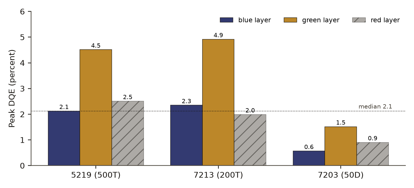
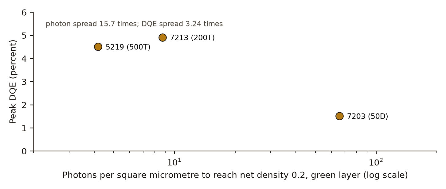
Reading three Kodak VISION3 data sheets as if the film were a photon counter, the best layer uses about 5 percent of the light's information and the median layer about 2 percent. In the green layer the 500T and 200T stocks match within 10 percent (4.5 and 4.9 percent) although one needs about twice the photons of the other; their blue layers differ by 11 percent and their red layers by 26.
- Tier
- B, signal
- Outcome
- held
- Rung
- hypothesis
- Verdicts
- 6 passed, 6 failed
- Corrections
- 3, latest 2026-11-14
- Version
- v3, 2026-11-14
- Redo it
- Reproduce
Download PDF 506 KB BuildTeX source F147.bld
What this means for a reader
Modern colour negative film keeps a few percent of the information in the light that reaches it, by this estimate at most about 5 percent in its best layer. That puts a number on film that can be set beside a sensor or an eye. For anyone who emulates film grain, the sheets themselves give a measured noise curve per layer, and that curve does not grow with density the way the textbook rule says.
Objection
One maker, one aperture, and vendor curves read from printed sheets. Digitising adds its own error, which was not measured.
What would change the call. Read Shaw and Dainty; measure one stock with a spectral photon count and a lab microdensitometer.
From the paper's first stated limitation; our register records no separate objection.
Abstract
Detective quantum efficiency asks how much of the information in arriving light a detector keeps, and it puts a film, a camera sensor and an eye on one scale. We derived it for the nine colour layers of three current Kodak motion-picture stocks, 5219 (500T), 7213 (200T) and 7203 (50D), from numbers Kodak prints on its data sheets, under a preregistered plan with planted checks. Peak detective quantum efficiency across the nine layers has a median of 2.1 percent and a range of 0.57 to 4.92 percent, an upper estimate because every photon is counted at the layer's most efficient wavelength. In the green layer, 500T and 200T reach 4.5 and 4.9 percent although 200T needs about twice the photons; 50D needs 15.7 times the photons of 500T and reaches 1.5 percent. Siedentopf's rule, that grain variance grows with density, lost on held-out points in 9 of 9 layers, and variance falls with density overall (median power slope -0.54); because our planted variance check failed, this is description only. A straight hinge in log exposure was the best held-out response form in 9 of 9 layers. A single Poisson hit-threshold model does not fit.
c1 observed, evidence for claim 1
- The numbers in claim 1
- 2.1; 0.57; 4.92 matches the result file, 2026-11-09
- Chart 2
- Peak DQE of each colour layer in three film stocks.
- Basis
- observed: measured in this study, with a result file
c2 observed, evidence for claim 2
- The numbers in claim 2
- 500; 200; 4.5; 4.9; 50; 15.7; 1.5 matches the result file, 2026-11-09
- Chart 3
- Green layer: light needed against information kept.
- Basis
- observed: measured in this study, with a result file
c3 observed, evidence for claim 3
- The numbers in claim 3
- 9; -0.54 matches the result file, 2026-11-09
- Chart 4
- How grain variance changes with density in each layer.
- Basis
- observed: measured in this study, with a result file
c4 observed, evidence for claim 4
- The numbers in claim 4
- 9 matches the result file, 2026-11-09
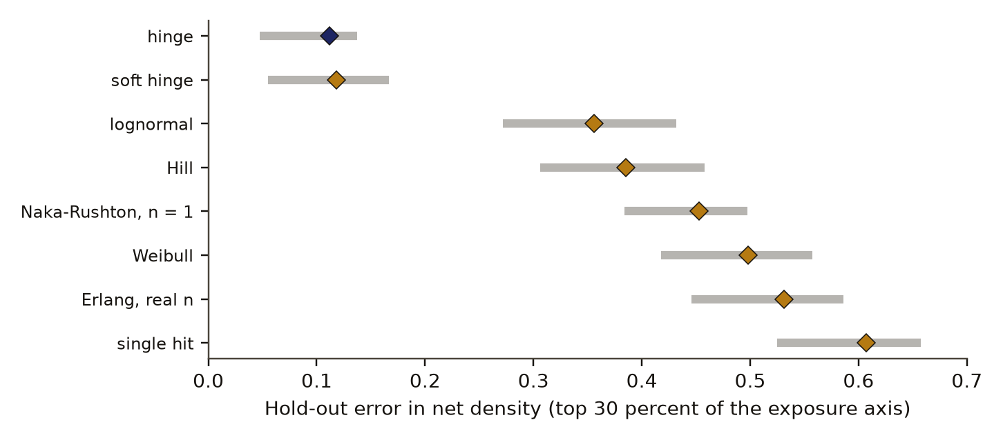
- Chart 5
- Hold-out error of eight response forms over the nine layers.
- Basis
- observed: measured in this study, with a result file
Introduction and motivation
A film is a photon detector with a long history of measurement. The detective quantum efficiency (DQE)Definition: detective quantum efficiency (DQE) imaging science and detector physics The share of the information carried by the arriving photons that a detector's output keeps, measured as the square of its output signal-to-noise ratio divided by the square of the input's. 1 is a perfect photon counter. Excludes the plain share of photons absorbed, and the speed of a film. full definition of a detector compares the information in its output with the information in the light that arrived. Shaw introduced the photographic form of the idea in 1963 under the name equivalent quantum efficiency [2] and used it to compare the information capacity of photography with other detectors [3]. Dainty and Shaw's book on image science [4] treats DQE curves, granularity and the characteristic curve together. We found these works through searches run on 9 November 2026 and read the abstract of the second Shaw paper and the catalogue records of the others; the full texts were not read.
What a sheet gives is enough for a ceiling estimate. Kodak publishes, for each colour layer, the characteristic curveDefinition: characteristic curve photographic sensitometry; also called the H and D curve The developed optical density of a film plotted against the logarithm of the exposure it received. Excludes the film's spectral sensitivity and its grain. full definition, the rms granularityDefinition: rms granularity photographic sensitometry The standard deviation of density read through a small round aperture scanned across a uniformly exposed patch. Kodak's sheets use a 48 micrometre aperture. Excludes how grainy the image looks to a viewer, and noise measured at other apertures. full definition against density, and the spectral sensitivityDefinition: spectral sensitivity photographic sensitometry For each wavelength, the reciprocal of the exposure energy per unit area needed to reach a stated net density, here 0.2. Excludes sensitivity to white light or to a named illuminant. full definition. From the first two come the noise-equivalent quanta (NEQ)Definition: noise-equivalent quanta (NEQ) imaging science The number of photons a perfect detector would need to give the same signal-to-noise ratio as the real output. Excludes the number of photons that arrived. full definition; from the third comes the number of photons. Their ratio is the DQE. A search summary we could not trace to a primary source put the best older films near 1 percent. We found no published DQE for the VISION3 stocks; that is what our searches returned, and it does not show that none exists.
The same sheets bear on two working rules. Siedentopf's ruleDefinition: Siedentopf's rule photographic science The classic statement that the variance of density grows in proportion to the mean density, so that rms granularity grows as its square root. Excludes Selwyn's law, which concerns the size of the measuring aperture. full definition says the variance of density grows in proportion to mean density, and it is the basis of signal-dependent grain models used in film emulation; Stephenson's grain simulation states it together with Selwyn's aperture law [5]. And a Poisson threshold modelDefinition: Poisson threshold model photographic science and visual physiology A model in which each grain, or each rod cell, responds once it has absorbed at least n photons, with photon counts following Poisson statistics. N is the hit number. Excludes models in which response grows smoothly with every photon. full definition, in which a grain develops after it absorbs n photons, has been used for both grains and rod cells in the eye. The study asked whether one such model describes the response and the noise of layered colour film together.
Preregistration and design
The plan was written and hash-locked in a preregistrationDefinition: preregistration research method (metascience) A dated written plan for a study, fixed and hash-locked before any result is seen: the question, the data, the statistic, the controls, the forecasts and the kill conditions. Excludes a plan revised after looking at the outcome, and a protocol written only for the record after the run. full definition on 31 October 2026 at 06:12:46 UTC, and the run followed at 06:12:48. It names the data, the measures, the planted checksDefinition: planted check research method; called a positive control in experimental science Data built so that the right answer is known, run through the same analysis before the real data, to show that the analysis can see the effect when it is there. Excludes any check made on the real data, which cannot show what the analysis misses. full definition, two controlsDefinition: control statistics and experimental design A version of the data with the structure under test removed (for example shuffled or pooled), scored the same way as the real data, so the real score has something to beat. Excludes a comparison with a different dataset or with a published number. full definition, the forecasts and the kill conditionsDefinition: kill condition research method (our usage, after Popper's falsification) A rule written in the preregistration that, when met, decides against the claim with no room for judgement after the run. Excludes reasons found after the run for setting a result aside. full definition. The decision it informs is what the grain and response parts of our film renderer should use.
One disclosure comes from the file itself. Before the lock, the 5219 stored curves had been looked at and one hand calculation had been made for the 5219 green layer, giving a DQE of about 0.11 with assumed values of gamma and sigma. So the forecasts for 5219 were not blind. The stocks 7203 and 7213 had been looked at only for calibration.
The rules that decide each verdictDefinition: verdict research method (our usage) The pass or fail of one preregistered rule set against the run's numbers, read off by code. Excludes an interpretation written after reading the numbers. full definition were written into the run's plan before the run. Any failed planted check voids its block. The full list is in Appendix A.
Data and provenance
The data are the Kodak VISION3 technical data sheets for 5219 (500T), 7213 (200T) and 7203 (50D) [1]. The curves were digitised from the published vector sheets: for each of the blue, green and red layers, the characteristic curve, the diffuse rms granularity curve measured with a 48 micrometre aperture, and the spectral sensitivity curve at a net densityDefinition: net density photographic sensitometry Optical density above the film's base and fog, so that unexposed film reads zero. Excludes the density of the base and the fog themselves. full definition of 0.2. The curves were resampled to a grid of 0.05 in log exposure. The sheets are Kodak's copyright. This paper reports only values derived from them and redraws none of their curves.
Kodak notes that its granularity figures use a modified measuring technique. We did not correct for it.
Methods
Photons
For each layer, let be the sheet's spectral sensitivity at the layer's peak wavelength , in reciprocal erg per square centimetre, at net density 0.2. The exposure that reaches net density 0.2 is , and dividing by the energy of one photon at gives the photon count per unit area there:
with Planck's constant and the speed of light, converted to photons per square micrometre. Counting every photon at the most efficient wavelength makes the fewest photons that could give net density 0.2, and so makes the DQE below an upper estimate.
At log exposure , the photons inside the 48 micrometre aperture, of area , are
where is the log exposure at which the curve reaches net density 0.2.
Noise-equivalent quanta and DQE
Let be the gammaDefinition: gamma photographic sensitometry The local slope of the characteristic curve: the change in density per unit change in log exposure. Excludes the display gamma of video and computer screens. full definition of the curve at , taken from a smoothed derivative, and the rms granularity at the same point. Then
Each layer's peak DQE is the largest value of eq. 4 over points with net density and gamma both above 0.05.
Grain variance
For points with net density above 0.1, four laws for the variance were compared: Siedentopf's , a constant, an affine law and a quadratic. Each was scored by BICDefinition: BIC statistics; the Bayesian information criterion A model score that adds a penalty for each fitted parameter to the misfit, lower being better, so that a more flexible model must earn its extra parameters. Excludes a test on held-out data. full definition on all points and by its hold-out scoreDefinition: hold-out score statistics and machine learning The error of a model fitted on one part of the data and scored on a part it never saw. Here fitted on the lowest 70 percent of the axis and scored on the top 30 percent. Excludes an error computed on the points used to fit. full definition in log variance on the top 30 percent of density after fitting on the rest. A power slope was fitted as
so that Siedentopf's rule corresponds to .
Response forms
Eight forms for net density against log exposure were fitted on the lowest 70 percent of the exposure axis and scored on the top 30 percent: Hill, Naka-Rushton with exponent 1, single hit, Erlang with real n, lognormal, Weibull, hingeDefinition: hinge curve fitting A response that is zero below a threshold exposure and rises in a straight line above it, here in log exposure. Excludes any form that saturates at high exposure. full definition and soft hinge. The hinge has two parameters, a threshold and a slope. BIC was reported beside the hold-out score, though the forms have different numbers of parameters.
Poisson threshold
The threshold model fits net density and log variance together, with hit number in 1, 2, 3, 4 and 6 and a lognormal spread of grain area with free width, and picks by BIC.
Controls and planted checks
Each block had a planted check with a known answer, run through the same code.
- DQE: synthetic single-size grains with a closed-form DQE. The pipeline came back within 11.3 percent, against a limit of 20. The DQE block stands.
- Response forms: five planted forms at the real data's scale of noise, 12 each, were recovered 80 percent of the time on hold-out, against a limit of 50. The forms block stands.
- Variance law: a planted affine law was chosen 70 percent of the time, against a locked requirement of 80. By the locked rule the variance verdict is voidDefinition: void research method (our usage) The verdict of a run whose planted check failed or whose sample fell below its stated minimum. It says nothing for or against the claim. Excludes a null result, which comes from a working instrument. full definition, and what we say about grain variance is description only.
c5 observed, evidence for claim 5
- Chart 1
- From a data sheet to a DQE, with a planted check on each block.
- Basis
- observed: measured in this study, with a result file
- Numbers
- None in the sentence; it reads the numbers stated beside it.
- dataThree curves per layerKodak prints a characteristic curve, a granularity curve and a spectral sensitivity curve for each colour layer.
- measurementPhotons, noise, DQESensitivity gives the photons that arrive. Slope and granularity give the photons the image is worth. The ratio is the DQE.
- measurementGrain variance and response formFour laws for variance against density and eight forms for density against exposure, each scored on held-out points.
- heldPlanted DQESynthetic grains with a known DQE came back within 0.113 of it. Limit 0.2.
- heldPlanted response formsPlanted forms were recovered on held-out points at a rate of 0.80. Limit 0.5 or more.
- failedPlanted variance lawThe planted law was chosen at a rate of 0.70. Required 0.8 or more. The variance verdict is void.
Read from result.json, run 20261031T061248Z. SHA-256 of the run's file 108b6952f1807a99580fdddd641ba3ca9dd38a3319f747becab8a60f168ad03a and of the published copy afa02962960df185b58f59d335e5b2a6bce1b86c2e40035f6a318ad430e6f3a5. In the copy, file paths are cut to the file name and the layout (indentation, line endings) may differ; every value is the same.
- Poisson threshold: planted hit numbers 1 and 4 were recovered every time at both grain widths, 0.5 and 2.0.
Two controls built a null distributionDefinition: null distribution statistics The spread of scores a control gives over many random draws. Its 95th percentile is the bar a real score must clear. Excludes a theoretical distribution assumed rather than drawn from the data. full definition for a statistic. Shuffling density against exposure 25 times gave a top-form share of 0.36 on average with a 95th percentile of 0.44; the real share of 1.0 is above all of them, a p value from drawsDefinition: p value (from draws) statistics The share of control draws scoring at or above the real score, with one added to the count and to the number of draws, so it is never zero. Excludes a p value from a textbook formula that assumes a distribution. full definition of 0.038, which is the smallest value 25 draws can give. Pairing one layer's slope with another layer's noise 200 times gave a mean correlation of 0.66 with a 95th percentile of 0.76; the real 0.61 sits inside it, p 0.74, so that test could not separate the layers.
The preregistration called for a Benjamini-Hochberg correctionDefinition: Benjamini-Hochberg correction statistics A rule for many tests at once: rank the p values from smallest, and reject the k smallest when the kth is no larger than k over the number of tests times the chosen false discovery rate, here 0.05. Excludes a correction for one test, and the stricter Bonferroni rule. full definition at 0.05 over the control p values. The result file does not report it. With two p values, 0.038 and 0.74, the smaller would have to be at or below 0.025 to pass, and it is not, so after the correction neither control rejects. The hinge result rests on its hold-out errors, which Figure 3 shows, more than on the shuffle.
Results
Peak detective quantum efficiency across the nine layers has a median of 2.1 percent and a range of 0.57 to 4.92 percent, an upper estimate because every photon is counted at the layer's most efficient wavelength. Table 1 gives each layer and Figure 1 draws them. The peak falls low on the curve, at net density 0.06 to 0.31, in the toe.
In the green layer, 500T and 200T reach 4.5 and 4.9 percent although 200T needs about twice the photons; 50D needs 15.7 times the photons of 500T and reaches 1.5 percent. The preregistered rule for "same efficiency at every speed" asked for a DQE spread of at most 3 across the three green layers while photon counts spread by 5 or more. The photon spread was 15.7 and the DQE spread 3.24, so the rule failed narrowly. Figure 2 shows the three points.
peak DQE, percent
photons per square micrometre for net density 0.2, log scale
- 5219 (500T)
- 7213 (200T)
- 7203 (50D)
Data behind chart 3 4 rows
| Stock | Photons per square micrometre | Peak DQE, percent |
|---|---|---|
| 5219 (500T) | 4.2 | 4.51 |
| 7213 (200T) | 8.7 | 4.92 |
| 7203 (50D) | 65.8 | 1.52 |
| Spread, highest over lowest | 15.7 | 3.24 |
Read from result.json, run 20261031T061248Z. SHA-256 of the run's file 108b6952f1807a99580fdddd641ba3ca9dd38a3319f747becab8a60f168ad03a and of the published copy afa02962960df185b58f59d335e5b2a6bce1b86c2e40035f6a318ad430e6f3a5. In the copy, file paths are cut to the file name and the layout (indentation, line endings) may differ; every value is the same.
Siedentopf's rule, that grain variance grows with density, lost on held-out points in 9 of 9 layers, and variance falls with density overall (median power slope -0.54); because our planted variance check failed, this is description only. The forecast slope was +0.15. The variance curves also show a hump in the toe. Our guess at a cause, untested, is the hand-off between fast and slow emulsions in a layered coating together with the colour masking couplers.
A straight hinge in log exposure was the best held-out response form in 9 of 9 layers. Its median hold-out error was 0.112 in net density, and every form that saturates did worse, as Figure 3 shows. Negative stock shows no shoulder within the range a sheet covers, so a form that bends over at high exposure loses when it extrapolates. Hill's exponent, fitted anyway, had a median of 0.615, which here is the gamma in another guise.
hold-out error in net density
- median over the nine layers
- lowest to highest layer
Data behind chart 5 8 rows
| Form | Median error | Lowest | Highest | Layers where it was best |
|---|---|---|---|---|
| Hinge | 0.112 | 0.047 | 0.137 | 9 |
| Soft hinge | 0.118 | 0.055 | 0.166 | 0 |
| Lognormal | 0.356 | 0.272 | 0.431 | 0 |
| Hill | 0.385 | 0.306 | 0.458 | 0 |
| Naka-Rushton, n = 1 | 0.453 | 0.384 | 0.497 | 0 |
| Weibull | 0.498 | 0.418 | 0.557 | 0 |
| Erlang, real n | 0.532 | 0.446 | 0.586 | 0 |
| Single hit | 0.607 | 0.525 | 0.658 | 0 |
Read from result.json, run 20261031T061248Z. SHA-256 of the run's file 108b6952f1807a99580fdddd641ba3ca9dd38a3319f747becab8a60f168ad03a and of the published copy afa02962960df185b58f59d335e5b2a6bce1b86c2e40035f6a318ad430e6f3a5. In the copy, file paths are cut to the file name and the layout (indentation, line endings) may differ; every value is the same.
The Poisson threshold model does not fit. On the channel the run used, the median error was 0.134 in log variance and 0.043 in density, against limits of 0.05 and 0.04. A later study of ours found that this fit passed the logarithm of the standard deviation where the model expected the logarithm of the variance. On the corrected channel the errors are 0.186 and 0.068, and the best hit number per layer changes from 1, 1, 1, 6, 6, 6, 6, 6, 6 to 1, 1, 1, 1, 6, 1, 6, 1, 1. The verdict stands either way, and no hit number is read as a measurement.
Discussion
The DQE figures sit above the roughly 1 percent we saw quoted for older films, and the planted grains show the pipeline itself is good to about 11 percent. Counting photons at the peak wavelength pushes every value up. Two other choices move them by an amount and in a direction we did not measure: the single aperture with Kodak's modified technique, and the toe, where gamma is small, so that a small error in the digitised slope is a large share of it, and NEQ goes as the square of gamma. The order of magnitude, a few percent, is the safer reading than any one figure.
The green layers carry the clearest pattern. 500T and 200T keep the same share of the information while one needs half the light of the other. A faster film here buys speed by needing fewer photons for the same density, and it does not lose efficiency doing so. 50D breaks the pattern at 1.5 percent. One stock is not enough to say why.
For a film renderer the decision is plain. Grain should come from each layer's measured granularity against exposure, with no square-root-of-density rule, and the response of negative stock within the sheet's range needs no saturating shoulder.
The threshold result connects to a later study of ours on rod cells, which found that rods and film grain do not share one threshold model on the data available. Nothing in this paper bears on rods.
Limitations
- One maker, one aperture, and vendor curves read from printed sheets. Digitising adds its own error, which was not measured.
- The photon count assumes all light at the peak wavelength, so every DQE here is an upper estimate. No interval is reported for the DQE values; the planted error of 11.3 percent is the only measure of the pipeline's accuracy.
- The variance verdict is void by our own rule. The variance results are description.
- The Benjamini-Hochberg correction the plan called for was not run; done by hand above, neither control survives it.
- Forecasts for 5219 were not blind, as the preregistration states.
- Shaw's 1963 papers and Dainty and Shaw's book were not read beyond abstracts and catalogue records, and may already set these numbers in context.
- Scoring was done by our own code and was not blind.
Evidence
Held. The quantum-efficiency part was calibrated on planted grains, and we found no published VISION3 figure. It rests on digitised vendor sheets, one aperture and a photon count at the peak wavelength. The planted variance check failed, the threshold-model fit failed, and the books by Shaw and by Dainty remain unread.
Figures
These are the paper's own figures, numbered as in the PDF, and each "Figure" reference in the text points here. The charts on this page redraw the same results from the result files and carry their own numbers.
Tables
| Stock | Layer | Photons | Peak DQE, percent | Net density at peak | Gamma at peak | Variance slope b | Hinge error |
|---|---|---|---|---|---|---|---|
| 5219 | blue | 1.2 | 2.12 | 0.26 | 0.55 | -0.66 | 0.096 |
| 5219 | green | 4.2 | 4.51 | 0.31 | 0.64 | -0.54 | 0.112 |
| 5219 | red | 10.8 | 2.51 | 0.12 | 0.44 | -0.51 | 0.117 |
| 7213 | blue | 2.9 | 2.35 | 0.29 | 0.60 | -0.32 | 0.047 |
| 7213 | green | 8.7 | 4.92 | 0.24 | 0.65 | -0.49 | 0.071 |
| 7213 | red | 20.2 | 1.99 | 0.16 | 0.55 | -0.56 | 0.054 |
| 7203 | blue | 33.6 | 0.57 | 0.14 | 0.46 | -0.59 | 0.137 |
| 7203 | green | 65.8 | 1.52 | 0.06 | 0.37 | -0.36 | 0.137 |
| 7203 | red | 87.6 | 0.90 | 0.17 | 0.54 | -0.71 | 0.132 |
Appendix A. The preregistered verdicts
Each verdict is a set of rules written before the run. A verdict passes only when every rule holds. Values are read from the run's result file.
| Verdict | Deciding rule | Value | Holds |
|---|---|---|---|
| Planted DQE | planted error at most 0.2 | 0.113 | yes |
| Planted variance law | planted law chosen at rate 0.8 or more | 0.70 | no |
| Planted forms | hold-out recovery 0.5 or more | 0.80 | yes |
| Siedentopf fails | beaten share 0.7 or more, and slope b below 0.7 | 1.0; -0.54 | yes, void |
| DQE in range | median peak DQE above 0.01 and below 0.2 | 0.021 | yes |
| Same efficiency at every speed | green DQE spread at most 3, and photon spread 5 or more | 3.24; 15.7 | no |
| No one form wins | top-form share below 0.6 | 1.0 | no |
| Form beats shuffled density | top-form share above the shuffle 95th percentile (0.44) | 1.0 | yes |
| Hit number unidentified, wide grains | planted recovery below 0.5 at width 2.0 | 1.0 | no |
| Hit number recovered, narrow grains | planted recovery 0.7 or more at width 0.5 | 1.0 | yes |
| Threshold form fits | density error at most 0.04, and log variance error at most 0.05 | 0.043; 0.134 | no |
| Slope tracks noise | median correlation above the pairing 95th percentile (0.76) | 0.61 | no |
Numbers recorded in our publication register
| What | Value |
|---|---|
| Sample | 3 stocks, 9 layers, one maker |
| Main estimate and interval | none reported for peak efficiency; planted error 0.11 |
| Forecast against outcome | median peak efficiency forecast 0.05, got 0.021; spread of green-layer efficiency across stocks forecast 2, got 3.24; variance slope forecast 0.15, got -0.54 |
| Known-answer check | planted closed-form grains recovered within 11 percent; planted hit numbers recovered in every case |
As recorded in the publication register, the summary row each finding gets; the paper's own numbers above were re-read from the result files.
What lowers it
- blinding Not blind. One hand calculation on the 5219 stock was made before the lock, as the paper states. from our publication register, on blinding
- failed check Controls: the planted checks on quantum efficiency and on response forms worked; the planted variance check failed (0.70 against 0.80), so the variance verdict is not credited; the pairing control did not separate. from our publication register, on controls
- novelty Nearby work exists; novelty is not shown. from our publication register, on the literature
- depth of reading The cited literature was read at the level of abstracts and catalogue records; full texts were not read. from the Verified section
What holds it up
- scoring Scored by code against rules fixed in advance. from our publication register, on who scored it
- preregistration Preregistered and hash-locked before the run (sha256 c0dbcacf). from the Reproduce section
- replication Rechecked by F164 (film hinge within the sheet's range): The hinge sits within the sheet's range, as F147 said, now on BIC. from a later finding
Where the claim stands
- lead
- hypothesis
- thesis
- conjecture
- theorem
- law candidate
- killed
A preregistration with pass-or-fail rules is on file, which this rung needs. The next rung needs a named rival reading beaten by a decisive observation, and none is on file. Tier B: The quantum-efficiency part was calibrated on planted grains, and we found no published VISION3 figure. It rests on digitised vendor sheets, one aperture and a photon count at the peak wavelength. The planted variance check failed, the threshold-model fit failed, and the books by Shaw and by Dainty remain unread.
Trail
Versions
- v3 2026-11-14, this page corrected, 1 item; the PDF and its BuildTeX source are still paper version 1.0
- v2 2026-11-09, paper version 1.0, first published PDF sha256 91f5daaa7942c3c1
- v1 2026-10-31, entered in the findings ledger
Corrections
2026-11-14 scope found by a review of the published pages
A review of the published page found the summary under the title wider than the result file supports. now It said the 500T and 200T stocks match within 10 percent; the file gives that for the green layer only (4.51 and 4.92 percent), with blue at 2.12 and 2.35 and red at 2.51 and 1.99. The summary now names the layer.
2026-11-09 wording found by the publication pass
The Benjamini-Hochberg step named in the preregistration was not run by the study. now This paper states the outcome it would have had.
2026-10-31 number found by a later study of ours
A later study of ours found that the Poisson threshold fit used log standard deviation where the model expected log variance. now Corrected errors 0.186 and 0.068; the failed verdict stands and the pattern of hit numbers changes, as given in the results.
Standing, and the ledger entries it rests on
2026-10-31 narrowed in part F163
Set by hand from findings ledger entry F163, dated 2026-10-31: film fit and its planted recovery. Rests on findings ledger, F163.
2026-10-31 held F164
Set by hand from findings ledger entry F164, dated 2026-10-31: film hinge within the sheet's range. Rests on findings ledger, F164.
Each correction is a dated note; the findings ledger is never rewritten, and a note governs where it differs.
Ledger and version dates up to publication are local dates in US Pacific time. Clock times in the text are UTC, seven or eight hours ahead, so a lock or a run stamped just after midnight UTC belongs to the previous local day. Corrections from 14 November 2026 on are dated in UTC.
References
- Eastman Kodak Company. KODAK VISION3 500T 5219, 200T 7213 and 50D 7203 colour negative films, technical data sheets. Example: https://www.kodak.com/content/products-brochures/motion-picture/KODAK-VISION3-500T-5219-7219-brochure.pdf run here Licence: Kodak sheets digitised; copyright terms apply, derived values only used in Data and provenance
- Shaw, R. (1963). The equivalent quantum efficiency of the photographic process. The Journal of Photographic Science 11, 199-204. doi:10.1080/00223638.1963.11736919 abstract or summary, 2026-11-09: abstracts and catalogue records; full text not read used in Introduction and motivation
- Shaw, R. (1963). Photon fluctuations, equivalent quantum efficiency, and the information capacity of photographic images. The Journal of Photographic Science 11(6), 313-320. doi:10.1080/00223638.1963.11736937 abstract or summary, 2026-11-09: abstracts and catalogue records; full text not read used in Introduction and motivation
- Dainty, J. C. and Shaw, R. (1974). Image Science: Principles, Analysis and Evaluation of Photographic-Type Imaging Processes. London: Academic Press. ISBN 0122008502. abstract or summary, 2026-11-09: abstracts and catalogue records; full text not read used in Introduction and motivation
- Stephenson, I. (2007). Simulating film grain using the noise power spectrum. Theory and Practice of Computer Graphics, Eurographics UK. abstract or summary, 2026-11-09: abstracts and catalogue records; full text not read used in Introduction and motivation
Cited by later findings
- F163 narrowed in part, film fit and its planted recovery, 2026-10-31 (record findings ledger, F163). The film fit passed log10 sigma into a model of log10 variance. On true variance the errors are 0.186 and 0.068; the failed verdict stands and the pattern of hit numbers changes.
- F164 held, film hinge within the sheet's range, 2026-10-31 (record findings ledger, F164). The hinge sits within the sheet's range, as F147 said, now on BIC.
Reproduce
Data
- Eastman Kodak Company. Licence: Kodak sheets digitised; copyright terms apply, derived values only. https://www.kodak.com/content/products-brochures/motion-picture/KODAK-VISION3-500T-5219-7219-brochure.pdf
Preregistration
sha256 c0dbcacf4caf6bd35564dde5fd02ea7b651165162206b5b1c4565fd9d326329a
plan 67bcd757fe62d97c70fef6dc556bc91e443a0842712cff5345841a4726373faa
Steps
- Data: the Kodak VISION3 technical data sheets for 5219, 7213 and 7203 [1], from Kodak's motion-picture product pages.
- Digitise, for each layer, the characteristic curve, the diffuse rms granularity curve at the 48 micrometre aperture and the spectral sensitivity at net density 0.2. Resample to 0.05 in log exposure.
- Compute eqs. 1, 2, 3 and 4 on that grid and take each layer's peak.
- Fit the variance laws, eq. 5, the eight response forms and the threshold model as in the methods, using log variance and not log standard deviation in the threshold fit.
- Preregistration SHA-256: c0dbcacf4caf6bd35564dde5fd02ea7b651165162206b5b1c4565fd9d326329a. Plan SHA-256: 67bcd757fe62d97c70fef6dc556bc91e443a0842712cff5345841a4726373faa. Run 20261031T061248Z. Result file SHA-256: 108b6952f1807a99580fdddd641ba3ca9dd38a3319f747becab8a60f168ad03a. Digitised data SHA-256: f3ebb6174d4a9e0f36f01837a6860c934c7b8c6783826b6661080a8b65c81427.
Cost. About two and a half minutes on one desktop CPU (56 s analysis, 96 s shuffle control, under 1 s pairing control). The study was not re-run for this paper.
Downloads
- Whitepaper, PDF F147.pdf, 506 KB
- BuildTeX source F147.bld, 31 KB
- Build receipt F147.buildtex.json, 1 KB
- BuildLang doc module doc.bld, 5 KB, imported by the source
The PDF is typeset by BuildTeX from F147.bld, which is written from the same source as this page. The receipt records the source's SHA-256 and the PDF's (91f5daaa7942), so anyone can rebuild it and compare. The copy here has its hidden author field blanked, as the site does for every file it publishes; blank the same field in a rebuild before comparing. The name stays on the first page.
Verified
Verified on 2026-11-09. On 9 November 2026 the nine peak DQE values (0.0057 to 0.0492, median 0.0212), the per-layer values in Table 1, the green-layer DQE and photon counts, the 3.24 and 15.7 spreads, the median slope -0.54, the planted results (0.113, 0.70, 0.80, 1.0), both controls and every verdict in Appendix A were re-read from the run's result file. They match the findings ledgerDefinition: findings ledger our records The append-only, dated list of every result we have recorded, numbered F1, F2 and on. Corrections are added as new dated lines and old entries are never rewritten. Excludes a curated list of successes. full definition. The preregistration's SHA-256 was recomputed from the file and matches the hash recorded in the lock and the run manifest. All three figures were drawn by a script that reads only the result file.
Not checked. The Poisson threshold values on the corrected channel come from the later ledger entry and were not recomputed here. The study was not re-run for this paper. The cited works were found by searches run on 9 November 2026 and read at the level of abstracts and catalogue records; their full texts were not read.
Terms on this page
Each term is defined where it is first used on this page. Each name below opens its entry in the findings glossary, which lists every page that uses it.
- detective quantum efficiency (DQE) imaging science and detector physics first use
- characteristic curve photographic sensitometry; also called the H and D curve first use
- rms granularity photographic sensitometry first use
- spectral sensitivity photographic sensitometry first use
- noise-equivalent quanta (NEQ) imaging science first use
- Siedentopf's rule photographic science first use
- Poisson threshold model photographic science and visual physiology first use
- preregistration research method (metascience) first use
- planted check research method; called a positive control in experimental science first use
- control statistics and experimental design first use
- kill condition research method (our usage, after Popper's falsification) first use
- verdict research method (our usage) first use
- net density photographic sensitometry first use
- gamma photographic sensitometry first use
- BIC statistics; the Bayesian information criterion first use
- hold-out score statistics and machine learning first use
- hinge curve fitting first use
- void research method (our usage) first use
- null distribution statistics first use
- p value (from draws) statistics first use
- Benjamini-Hochberg correction statistics first use
- findings ledger our records first use
To report an error, name the finding, the claim number and the source on the Work page, which gives the address. Accepted corrections join the Trail with their date.