
Findings F114 Plants, trees and earth, Biology and medicine, Information and signal found 2026-10-30
How much summer warmth one tree ring remembers, measured in bits
A single Alpine tree-ring site keeps about a tenth of a bit per year about summer warmth on years it never saw, most of it in the density of its latewood. Averaging many sites buys far more than adding a measurement or one more tree past the usual replication threshold.
- Tier
- B*, strong signal
- Outcome
- held
- Rung
- hypothesis
- Verdicts
- 5 passed, 2 failed
- Kill rule
- not fired
- Corrections
- 3, latest 2026-11-14
- Version
- v3, 2026-11-14
- Redo it
- Reproduce
Download PDF 574 KB BuildTeX source F114.bld
What this means for a reader
A single tree-ring site keeps about a tenth of a bit a year about summer warmth, and most of that sits in the density of its late wood. That ranking of density over width is old news to tree-ring scientists. What is new is one shared unit: a second measurement in the same trees, one more tree at a site and a network of sites can now be priced against each other, and the network wins by a wide margin.
Objection
Bits are a relabelling of the coefficient of efficiency, so what is new? Further: the regional gain partly reflects a smoother target, the null on the forecast that an added channel beats an added tree is underpowered, cores stand in for trees, cloud cover is interpolated, and the windows end near 1975.
What would change the call. Give the channel-against-tree test more power with wider panels and nested best-subset selection; an outside dendrochronologist's review; a band or period out of sample past 1975.
From the strongest objection recorded in our publication register.
Abstract
Tree rings hold several measurable records of each summer: the width of the ring, of its early and late wood, and the density of its wood. We put all of them on one scale, bits per year of summer climate recovered on years the model never saw, so that a new channel, a new tree and a new site can be compared directly. The data are 51 Alpine and 24 Fennoscandian sites from the International Tree-Ring Data Bank with five channels gap-free from 1901, and June to August climate from CRU TS 4.10. In the Alps, maximum latewood density kept 0.090 bits per year of summer warmth on held-out years and ring width 0.028; density beat width by 0.062 bits (95% interval 0.034 to 0.089). In Fennoscandia, density beat width by 0.28 bits (0.23 to 0.33). The gain from extra channels did not saturate by three: the saturation ratio was 0.25 against a forecast bound of 0.10. An added channel and one more tree past an expressed population signal of 0.85 could not be told apart: the difference was 0.011 bits (-0.003 to 0.025) over 43 sites. Averaging all 51 Alpine sites reconstructed summer warmth with a held-out coefficient of efficiency of 0.317, which is 0.275 bits per year. At one site a ring is a narrow channel. Most of the gain comes from averaging across sites.
c1 observed, evidence for claim 1
- The numbers in claim 1
- 0.090; 0.028; 0.062; 95; 0.034; 0.089 matches the result file, 2026-11-09
- Chart 2
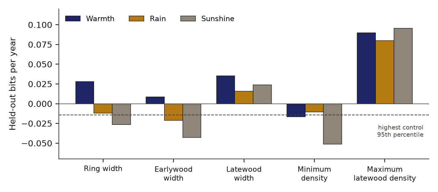
- Held-out bits per year about summer warmth, one ring channel at a time, in the Alps.
- Basis
- observed: measured in this study, with a result file
c2 observed, evidence for claim 2
- The numbers in claim 2
- 0.28; 0.23; 0.33 matches the result file, 2026-11-09
- Chart 5
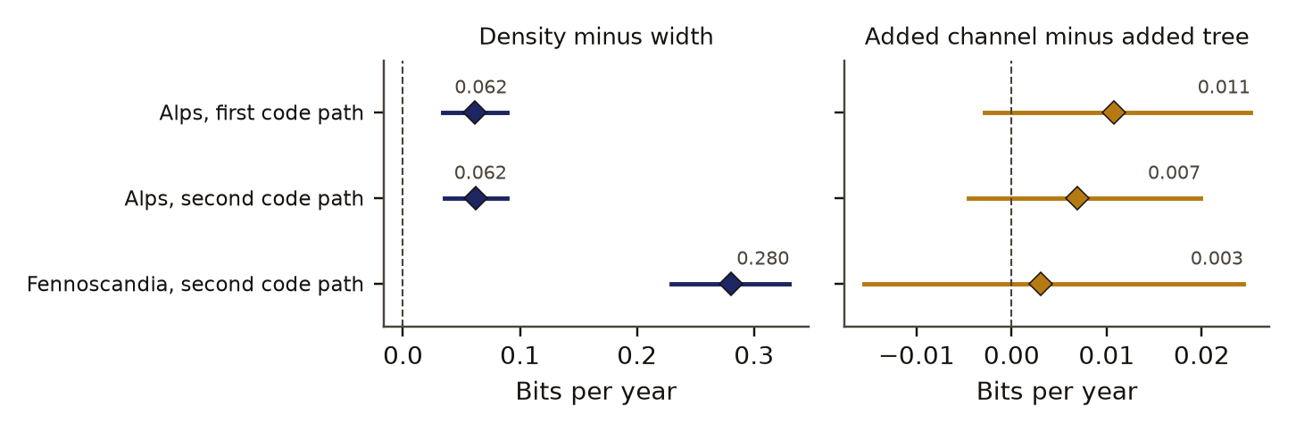
- Density minus width: how many more held-out bits about summer warmth density keeps, in two regions and two code paths.
- Basis
- observed: measured in this study, with a result file
c5 observed, evidence for claim 5
- The numbers in claim 5
- 0.25; 0.10 matches the result file, 2026-11-09
- Chart 3
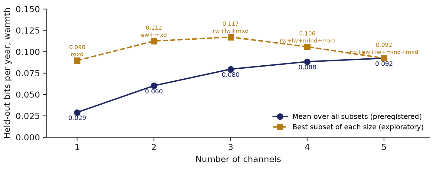
- Held-out bits about summer warmth against the number of ring channels used together, in the Alps.
- Basis
- observed: measured in this study, with a result file
c3 observed, evidence for claim 3
- The numbers in claim 3
- 0.85; 0.011; -0.003; 0.025; 43 matches the result file, 2026-11-09
- Chart 4
- One more channel against one more tree: the difference in held-out bits, in both regions.
- Basis
- observed: measured in this study, with a result file
c4 observed, evidence for claim 4
- The numbers in claim 4
- 51; 0.317; 0.275 matches the result file, 2026-11-09
- Basis
- observed: measured in this study, with a result file
Introduction
Dendroclimatology, the reading of past climate from tree rings, measures several ring channelsDefinition: ring channel dendrochronology, our usage after the channel of information theory One quantity measured in every annual ring of a site's trees and kept as a yearly series: ring width, earlywood width, latewood width, minimum density or maximum latewood density. Excludes a climate variable, and a combination of several measured quantities. full definition in each annual ring. For summer temperature at cold sites, maximum latewood densityDefinition: maximum latewood density dendrochronology (densitometry) The highest wood density in the late, dense part of an annual ring, read from an X-ray image of a thin lath of the core. Excludes ring width and the mean density of the whole ring. full definition has long been the stronger channel. Grudd [3] updated the Torneträsk width and density series in northern Sweden to cover AD 500 to 2004 and reported that a reconstruction from density captures 63 to 64 percent of the year-to-year variation in summer temperature. Römer and colleagues [4] compared eleven proxies measured in the same ten pines in Greece, including width, density, stable isotopes and cell anatomy, and reported their covariance and climate signals as correlations.
Replication is the other lever. Wigley, Briffa and Jones [1] derived how well the mean of a finite number of series stands for the population, the expressed population signalDefinition: expressed population signal (EPS) dendrochronology How well the mean of k series stands for the mean of an infinite set of such series, k r over 1 plus (k minus 1) r, with r the mean correlation between series. 0.85 is the conventional threshold. Excludes a measure of how well the series track climate. full definition. A value of 0.85 became the common threshold for enough trees. Buras [2] pointed out that the original paper offered its value only as a rough guide, so 0.85 is a convention.
These comparisons use correlation, and each answers one question at a time: which channel, or how many trees. Information theory offers a unit that adds across sources and does not depend on which question is asked. The bitDefinition: bit information theory The unit of information: one bit halves the uncertainty about an outcome, so a record that keeps b bits a year narrows each year's range of possible summers by a factor of 2 to the power b, as measured by its standard deviation. Excludes a count of stored numbers, and any statement about which way the dependence runs. full definition is that unit. Searches we ran on 9 November 2026 found no study that scores tree-ring channels against climate in bits; the closest work compares channels in correlation units. A search that finds nothing is a search result, not proof that nothing exists.
This paper asks four things. How many bits per year of summer warmth, rain and sunshine survive into each ring channel? What does each added channel buy? What does each added tree buy past an expressed population signal of 0.85? Can the season be reconstructed on held-out years?
Preregistration and design
The design was written and hash-locked as a preregistrationDefinition: preregistration research method (metascience) A dated written plan for a study, fixed and hash-locked before any result is seen: the question, the data, the statistic, the controls, the forecasts and the kill conditions. Excludes a plan revised after looking at the outcome, and a protocol written only for the record after the run. full definition on 30 October 2026 at 12:18 UTC, before any ring or climate outcome was computed. Site availability had been counted before the lock without looking at outcomes: 51 Alpine and 24 Fennoscandian sites, with median series lengths of 79 and 78 years.
The locked file names the data, the targets, the filter, the three measures, the planted signals with their pass rules, the three controlsDefinition: control statistics and experimental design A version of the data with the structure under test removed (for example shuffled or pooled), scored the same way as the real data, so the real score has something to beat. Excludes a comparison with a different dataset or with a published number. full definition, the kill conditionDefinition: kill condition research method (our usage, after Popper's falsification) A rule written in the preregistration that, when met, decides against the claim with no room for judgement after the run. Excludes reasons found after the run for setting a result aside. full definition, five predictions with their rules, the multiple-testing plan and a replication on Fennoscandia by a second code path. The kill condition: the study fails if no channel carries more than the controls, that is, if the best channel does not beat the 95th percentile of all three controls or no test survives correction.
Two deviations were recorded after the lock and before any outcome was seen. The first Alpine run stopped with an error inside the isotope step because one isotope site held six missing values that the parser read as numbers. The fix keeps only finite values, so that site fails the existing gap-free rule and leaves the isotope panel, which drops to 19 sites; the failed run printed no number. The second: the Alpine check by the second code path was blocked by our run tool because a shared file changed during that fix, and it was rerun unchanged. The plan hash did not change.
Data and provenance
Rings: International Tree-Ring Data Bank chronologies for Europe [8], held by NOAA's National Centers for Environmental Information as open federal data, with a request to cite the original study, landing page and access date. Five channels per site: ring width, earlywood width, latewood width, minimum density and maximum latewood density, with raw measurement files for width and density. A site entered when all five channels were gap-free from 1901 to their common end year, with at least 50 years. The Alpine box is 43.5 to 48.5 N and 5 to 17 E, and the Fennoscandian box is 58 to 71.5 N and 4 to 32 E. Most of these density sites come from the Schweingruber collection, so the series end about 1975 to 1990; the 51 Alpine windows used here run 74 to 82 years from 1901, so they end between 1974 and 1982.
Isotopes: ISONET latewood or whole-ring cellulose oxygen isotope chronologies [9], released under CC BY 4.0. 19 European sites with complete values from 1901 to 2002 were used.
Climate: CRU TS 4.10 monthly temperature, precipitation and cloud cover at 0.5 degree, 1901 to 2025 [6] [7], released under the Open Database License 1.0. Each site takes the nearest land cell with complete data. The targets are the June to August mean temperature (warmth), total precipitation (rain) and 100 minus mean cloud cover in percent (sunshine, a proxy for light).
Every channel and target series was passed through a high-pass filterDefinition: high-pass filter signal processing A filter that keeps fast variation and removes slow trends. Here each series minus a Gaussian smooth of width 10 years, which keeps roughly the 2 to 30 year band. Excludes a fixed polynomial detrend. full definition on its own window: the series minus a Gaussian smooth of width 10 years, renormalised at the edges, then scaled to zero mean and unit variance. The study therefore measures variation from 2 years to roughly 30 years.
Methods
Held-out bits
For each channel and target at a site, a linear reconstruction was fitted by block cross-validationDefinition: block cross-validation statistics and machine learning The years are split into contiguous blocks, here five. Each block in turn is held out, the model is fitted on the rest and scored on the held-out block. Excludes a score on the fitting years, and splits that scatter single years so that neighbouring years leak into the fit. full definition with five contiguous blocks. Let be the target in a held-out year, the reconstruction and the mean of the held-out years. The coefficient of efficiencyDefinition: coefficient of efficiency (CE) hydrology and dendroclimatology; also called the Nash-Sutcliffe efficiency One minus the mean squared error of a reconstruction on held-out years divided by the variance of the true values in those years. 1 is perfect and 0 means no better than the held-out years' own mean. Excludes a correlation, which ignores bias and scale errors. full definition is
and the held-out information in bits per year is
For a Gaussian target with variance , any predictor that carries bits of mutual informationDefinition: mutual information information theory The reduction in uncertainty about one variable from knowing another, in bits, which counts any dependence and not only linear dependence. Excludes a measure of the size of a slope or of causation. full definition has a mean squared error of at least . So is a lower bound on the information the ring carries, read off held-out years. It is negative when the reconstruction does worse than the held-out mean. The network value is the mean of over sites. Beside it we report the KSG estimatorDefinition: KSG estimator statistics and information theory The k-nearest-neighbour estimate of mutual information from samples given by Kraskov, Stoegbauer and Grassberger, here with 4 neighbours. Excludes estimates that first bin the data into histograms. full definition of mutual information [5] with 4 neighbours, and an in-sample Gaussian value from the correlation.
Channels, trees and sites
Prediction P1, density beats width: the 95% site bootstrapDefinition: site bootstrap statistics An interval made by recomputing a network mean many times on sites drawn with replacement from the panel, so the spread reflects differences between sites. Excludes an interval over years or over model refits at one site. full definition interval of the mean difference in between maximum latewood density and ring width for warmth lies above 0, the KSG difference is positive, and density survives correction.
Prediction P2, channels saturate by three: let be the mean of the network over all subsets of channels, and the larger of and . The saturation ratio is
and P2 passes if exceeds and is at most 0.10.
Prediction P3, a channel buys more than a tree: at each site, is the smallest number of density series whose expressed population signal reaches 0.85,
with the mean correlation between density series. The tree gain is the held-out bits of the mean of density series minus those of series. The channel gain is the bits of density and width means from the same series minus those of density alone. Each gain is averaged over 50 random draws of series. P3 passes if at least 10 sites qualify and the site bootstrap interval of the mean difference, channel gain minus tree gain, lies above 0. Each raw series is a core and stands in for a tree.
Prediction H4, the season can be reconstructed: the site means of each channel predict the regional warmth. It passes if the cross-validated is above 0, the reduction of errorDefinition: reduction of error (RE) dendroclimatology The same as the coefficient of efficiency, except that the reference is the mean of the calibration years, so it rewards getting a shift in mean right. Excludes a score computed on the years used to fit the model. full definition on a classic split (verify 1901 to 1930, calibrate 1931 to the end) is above 0, and beats the 95th percentile of 1,000 phase-randomisedDefinition: phase randomisation time-series statistics, surrogate data A copy of a series with the same power spectrum and random Fourier phases, so it keeps the series' autocorrelation and loses its timing against any other series. Excludes shuffling years, which also destroys the autocorrelation. full definition composites.
Prediction H5, isotopes carry climate: at least one of warmth, rain and sunshine survives correction on at the 19 isotope sites.
Controls, p values and correction
Three controls, 1,000 draws each, give the kill statistic's null distributionDefinition: null distribution statistics The spread of scores a control gives over many random draws. Its 95th percentile is the bar a real score must clear. Excludes a theoretical distribution assumed rather than drawn from the data. full definition: each site channel replaced by a phase-randomised copy; the years of each channel shuffled; and each channel replaced by high-passed white noise. The statistic is the largest network mean over the 15 channel and target tests. Each test's p value comes from 1,000 phase-randomised copies of the network mean, as a p value from drawsDefinition: p value (from draws) statistics The share of control draws scoring at or above the real score, with one added to the count and to the number of draws, so it is never zero. Excludes a p value from a textbook formula that assumes a distribution. full definition:
with the draws at or above the real value and the draws, so the smallest possible value is 0.001. The 15 tests of each measure, and the 3 isotope tests, were adjusted with the Benjamini-Hochberg correctionDefinition: Benjamini-Hochberg correction statistics, multiple testing A rule that adjusts a set of p values so that, among the tests called significant, the expected share of false calls stays at or below a chosen rate q, here 0.05. Excludes the stricter Bonferroni rule, which bounds the chance of any false call. full definition at q 0.05.
Second code path
A second program, written apart and sharing no code with the first, repeats the analysis with different filters, a k-d tree KSG, normal-equation cross-validation and full-length Fourier surrogates. It ran on the Alps as a check of the code and on Fennoscandia as a replication, with the same rules and without the isotope test. The replication passes when every primary verdict matches and, for the Alpine check, the P1 effect falls inside the first path's interval. A different region may differ, and any difference is reported as a result about that region.
Controls and planted checks
The planted checkDefinition: planted check research method; called a positive control in experimental science Data built so that the right answer is known, run through the same analysis before the real data, to show that the analysis can see the effect when it is there. Excludes any check made on the real data, which cannot show what the analysis misses. full definition ran in the same job, four synthetic sites per real site, on the panel's own series lengths. A target with year-to-year persistence of 0.3 was paired with a channel at correlation 0.6, which carries 0.322 bits. The planted 0.322 bits read 0.331 by the Gaussian value, 0.308 by KSG and 0.269 on held-out years. The held-out reading falls short of the truth, as a lower bound should, and inside the preregistered range. A second independent channel worth 0.222 bits more added 0.201 on held-out years. A white-noise channel scored -0.050 and a near-copy of the first channel added -0.012, so neither was mistaken for signal. Every anchor rule held.
c6 observed, evidence for claim 6
- The numbers in claim 6
- 0.322; 0.331; 0.308; 0.269 matches the result file, 2026-11-09
- Chart 1
- Planted check: a synthetic channel that carries a known number of bits, read by the three estimators.
- Basis
- observed: measured in this study, with a result file
On the real data the best test scored 0.095 bits, sunshine from maximum latewood density, against control 95th percentiles of -0.014 (phase), -0.017 (shuffle) and -0.017 (white noise), each with p 0.001. Of the 15 channel and target tests, 14 survived correction on held-out bits and 9 on KSG. Six of those 14 have negative held-out bits (the lowest is earlywood width for sunshine at -0.043): they score above the controls and still forecast worse than the held-out mean, so surviving the correction is not the same as carrying signal. The kill condition did not fire.
Results
One channel at a time
Table 1 and Figure 1 give the held-out bits of every channel in the Alps. In the Alps, maximum latewood density kept 0.090 bits per year of summer warmth on held-out years and ring width 0.028; density beat width by 0.062 bits (95% interval 0.034 to 0.089). The KSG difference was 0.067. Density also carried 0.080 bits about rain and 0.095 about sunshine. Earlywood width and minimum density carried little or nothing on held-out years.
More channels
The gain from extra channels did not saturate by three: the saturation ratio was 0.25 against a forecast bound of 0.10. The mean over subsets of each size ran 0.029, 0.060, 0.080, 0.088 and 0.092 bits for one to five channels, so P2 failed. The mean over subsets mixes two things: which channel is chosen and how many. The best subset of each size, which we did not preregister, peaked at three channels (0.117 bits, ring width, latewood width and density) and fell to 0.092 with all five. With about 80 summers per site, more than three channels overfit. Figure 2 shows both curves.
held-out bits per year about summer warmth
number of channels
- mean over all subsets of that size (set in advance)
- best subset of that size (not set in advance)
Data behind chart 3 5 rows
| Channels | Mean over subsets | Best subset | Channels in the best subset |
|---|---|---|---|
| 1 | 0.029 | 0.090 | maximum latewood density |
| 2 | 0.060 | 0.112 | earlywood width, maximum latewood density |
| 3 | 0.080 | 0.117 | ring width, latewood width, maximum latewood density |
| 4 | 0.088 | 0.106 | ring width, latewood width, minimum density, maximum latewood density |
| 5 | 0.092 | 0.092 | ring width, earlywood width, latewood width, minimum density, maximum latewood density |
Read from alps-result.json, run 20261030T123853Z. SHA-256 of the run's file 65d480942aad29a6838af7468aecf78184d00689b20182ec52689b79c53a1e63 and of the published copy 6c2dc1522416b198ece9e97d7a2ec689bb0f98a9b3a4acf23b394fa344eeb586. In the copy, file paths are cut to the file name and the layout (indentation, line endings) may differ; every value is the same.
A channel or a tree
An added channel and one more tree past an expressed population signal of 0.85 could not be told apart: the difference was 0.011 bits (-0.003 to 0.025) over 43 sites. The added channel gained 0.014 bits and the added tree 0.004. The median site needed 5 density series to reach 0.85. P3 failed, and its null is inconclusive: the interval is wide compared with both gains. Read as a curve, the held-out bits of density means rose from 0.044 with one series to 0.099 with 12, at the 29 sites that had 12 series.
channel gain minus tree gain, bits per year
- channel gain minus tree gain
- 95% site bootstrap interval
- no difference
Data behind chart 4 3 rows
| Run | Sites | Channel gain | Tree gain | Difference | Low | High |
|---|---|---|---|---|---|---|
| Alps, first code path | 43 | 0.014 | 0.004 | 0.011 | −0.003 | 0.025 |
| Alps, second code path | 42 | 0.010 | 0.003 | 0.007 | −0.005 | 0.020 |
| Fennoscandia, second code path | 23 | 0.018 | 0.015 | 0.003 | −0.016 | 0.024 |
Read from alps-result.json, run 20261030T123853Z. SHA-256 of the run's file 65d480942aad29a6838af7468aecf78184d00689b20182ec52689b79c53a1e63 and of the published copy 6c2dc1522416b198ece9e97d7a2ec689bb0f98a9b3a4acf23b394fa344eeb586. In the copy, file paths are cut to the file name and the layout (indentation, line endings) may differ; every value is the same.
Read from alps-second-path-result.json, run 20261030T124501Z. SHA-256 of the run's file 5f6ba9957994f12b3cf511994e22a87bb6b3c32b06628e05b2b4963325a6b565 and of the published copy fb088c9c81631751fca6aca5235e1220c4fde95550982f82abe4a4e4dadd0212. In the copy, file paths are cut to the file name and the layout (indentation, line endings) may differ; every value is the same.
Read from fennoscandia-result.json, run 20261030T123301Z. SHA-256 of the run's file d7e616aecfae261d49be8e9b33625a9e4469d55f702af4bd8464119269bb4cc0 and of the published copy 73e1c1f36809bb4dfd9b4cea5f2374fbe9e10336410f723c6df73eec44be7dbb. In the copy, file paths are cut to the file name and the layout (indentation, line endings) may differ; every value is the same.
Many sites
Averaging all 51 Alpine sites reconstructed summer warmth with a held-out coefficient of efficiency of 0.317, which is 0.275 bits per year. The reduction of error on the classic split was 0.391, and the phase-randomised composites' 95th percentile was 0.023, so H4 passed. The regional means reached 0.217 bits for rain and 0.168 for sunshine. By month, the five regional channels together gave held-out efficiencies of -0.03 in April, -0.06 in May, 0.17 in June, 0.16 in July and 0.27 in both August and September. Density alone gave 0.31 in August and 0.33 in September.
Isotopes
At the 19 European isotope sites, oxygen isotopes carried 0.052 bits of warmth, 0.102 of rain and 0.110 of sunshine on held-out years, and all three survived correction, so H5 passed.
The second code path and Fennoscandia
Table 2 and Figure 3 set the two code paths and the two regions side by side. On the Alps the second path gave the same six verdicts, and its P1 effect of 0.062 (0.035 to 0.089) sits inside the first path's interval. In Fennoscandia, density beat width by 0.28 bits (0.23 to 0.33). That is outside the Alpine interval: the same sign and a larger effect at the cold northern tree line. Regional warmth there was reconstructed with a held-out efficiency of 0.72, which is 0.93 bits. P2 and P3 failed in Fennoscandia as well. Maximum latewood density kept 0.24 bits about warmth there and -0.08 about sunshine, while in the Alps it kept about as much about sunshine (0.095) as about warmth (0.090).
density minus width, held-out bits per year
- density minus width
- 95% site bootstrap interval
- no difference
Data behind chart 5 3 rows
| Run | Sites | Density minus width | Low | High | Same difference by KSG | Saturation ratio |
|---|---|---|---|---|---|---|
| Alps, first code path | 51 | 0.062 | 0.034 | 0.089 | 0.067 | 0.25 |
| Alps, second code path | 51 | 0.062 | 0.035 | 0.089 | 0.084 | 0.23 |
| Fennoscandia, second code path | 24 | 0.280 | 0.229 | 0.330 | 0.186 | 0.54 |
Read from alps-result.json, run 20261030T123853Z. SHA-256 of the run's file 65d480942aad29a6838af7468aecf78184d00689b20182ec52689b79c53a1e63 and of the published copy 6c2dc1522416b198ece9e97d7a2ec689bb0f98a9b3a4acf23b394fa344eeb586. In the copy, file paths are cut to the file name and the layout (indentation, line endings) may differ; every value is the same.
Read from alps-second-path-result.json, run 20261030T124501Z. SHA-256 of the run's file 5f6ba9957994f12b3cf511994e22a87bb6b3c32b06628e05b2b4963325a6b565 and of the published copy fb088c9c81631751fca6aca5235e1220c4fde95550982f82abe4a4e4dadd0212. In the copy, file paths are cut to the file name and the layout (indentation, line endings) may differ; every value is the same.
Read from fennoscandia-result.json, run 20261030T123301Z. SHA-256 of the run's file d7e616aecfae261d49be8e9b33625a9e4469d55f702af4bd8464119269bb4cc0 and of the published copy 73e1c1f36809bb4dfd9b4cea5f2374fbe9e10336410f723c6df73eec44be7dbb. In the copy, file paths are cut to the file name and the layout (indentation, line endings) may differ; every value is the same.
Discussion
On one shared scale the ranking is plain. A site's densest latewood keeps about three times what its ring width keeps about summer warmth, and at the northern tree line the gap is larger. This agrees with what Grudd [3] and Römer and colleagues [4] report in correlation units. The unit adds one thing: the second channel, the extra tree and the site network can be compared directly.
Read that way, a ring at one site is a narrow channel, about a tenth of a bit a year. A second channel in the same trees and one more tree past the usual replication threshold both buy around a hundredth of a bit, and we could not tell them apart. Averaging 51 sites buys about three times what the best single channel keeps at one site. Part of that gain is a property of the target: a regional mean of summer warmth is smoother than the climate at one grid cell, so it is easier to predict.
The failed saturation forecast has a plain cause. The mean over subsets of a given size includes the weak channels, so it keeps rising as the chance of including density rises. The best subset peaks at three channels, as we forecast, but that curve was not preregistered and is reported as exploration. Next time the best-subset curve, with the subset chosen inside each fold, should be the registered one.
The tree-against-channel comparison follows Wigley, Briffa and Jones [1]. Past an expressed population signal of 0.85, another tree adds little, which is what the threshold is meant to say. Our run did not have the power to show that a second channel adds more.
Limitations
- Bits here are a monotone function of the coefficient of efficiency, so the unit relabels a familiar skill score. Its value is that channels, trees and sites share one scale.
- The ranking of density over width is long known.
- Part of the regional gain comes from a smoother regional target.
- The channel against tree comparison is underpowered, and its null is inconclusive.
- Cores stand in for trees.
- CRU cloud cover is partly interpolated and relaxed toward climatology where stations are sparse, so the sunshine bits are a floor.
- The windows end about 1975, and early CRU data are thin.
- The held-out bits are a lower bound for a near-Gaussian target, and the targets cover June to August, the 2 to 30 year band and one grid cell per site.
- The isotope panel is Europe-wide, not Alpine. The carbon isotope set could not be downloaded and was not used.
- Scoring was done by our own code and was not blind.
Evidence
Held. Real data, a preregistration, a planted check with a known answer, working controls and a second code path in a second region. Bits are a monotone transform of the coefficient of efficiency, and the ranking of density over width is long known. The comparison of an added channel with an added tree is an inconclusive null.
Figures
These are the paper's own figures, numbered as in the PDF, and each "Figure" reference in the text points here. The charts on this page redraw the same results from the result files and carry their own numbers.
Tables
| Channel | Warmth | Rain | Sunshine | KSG, warmth |
|---|---|---|---|---|
| Ring width | 0.028 | -0.012 | -0.026 | 0.038 |
| Earlywood width | 0.009 | -0.021 | -0.043 | 0.037 |
| Latewood width | 0.035 | 0.016 | 0.024 | 0.063 |
| Minimum density | -0.016 | -0.010 | -0.051 | 0.006 |
| Maximum latewood density | 0.090 | 0.080 | 0.095 | 0.105 |
| Quantity | Alps, first path | Alps, second path | Fennoscandia, second path |
|---|---|---|---|
| Sites | 51 | 51 | 24 |
| Density minus width, bits | 0.062 (0.034 to 0.089) | 0.062 (0.035 to 0.089) | 0.280 (0.229 to 0.330) |
| Saturation ratio | 0.25 | 0.23 | 0.54 |
| Channel minus tree, bits | 0.011 (-0.003 to 0.025) | 0.007 (-0.005 to 0.020) | 0.003 (-0.016 to 0.024) |
| Sites for channel against tree | 43 | 42 | 23 |
| Regional held-out efficiency | 0.317 | 0.315 | 0.723 |
| Regional bits per year | 0.275 | 0.273 | 0.927 |
| Tests surviving correction | 14 of 15 | 14 of 15 | 10 of 15 |
Appendix A. The preregistered verdicts
Each verdictDefinition: verdict research method (our usage) The pass or fail of one preregistered rule set against the run's numbers, read off by code. Excludes an interpretation written after reading the numbers. full definition is a set of rules written before the run, and it passes only when every rule holds. Values are from the Alpine result file.
| Verdict | Deciding rule | Value | Holds |
|---|---|---|---|
| Planted anchor | Gaussian error at most 0.04, KSG error at most 0.03, held-out reading within -0.12 to +0.02 of truth, pair gain at least 0.12, KSG pair error at most 0.10, white noise at most 0 and its KSG within 0.02, redundant gain at most 0 | 0.009; 0.014; -0.053; 0.201; 0.068; -0.050; 0.007; -0.012 | yes |
| Kill test survived | best test above all three controls' 95th percentiles; at least one test survives correction | 0.095 against -0.014; 14 | yes |
| P1 density beats width | interval lower end above 0; KSG difference above 0; density survives correction | 0.034; 0.067; yes | yes |
| P2 saturates by three | gain from one to three above 0; saturation ratio at most 0.10 | 0.051; 0.25 | no |
| P3 channel beats tree | at least 10 sites; interval lower end above 0 | 43; -0.003 | no |
| H4 season reconstructed | held-out efficiency above 0 and above the surrogate 95th percentile; split reduction of error above 0 | 0.317 against 0.023; 0.391 | yes |
| H5 isotopes carry climate | at least one of three targets survives correction | 3 | yes |
Numbers recorded in our publication register
| What | Value |
|---|---|
| Sample | 51 Alpine and 24 Fennoscandian sites, 74 to 78 regional years, 43 sites for the channel-against-tree test, 19 oxygen-isotope sites |
| Main estimate and interval | density minus width +0.062 bits (0.034 to 0.089); Fennoscandia +0.28 (0.23 to 0.33); added channel minus added tree 0.011 (-0.003 to 0.025) |
| Forecast against outcome | Passed: density beats width, the season forecast and the isotope forecast. Failed: saturation by three channels (ratio 0.25 against a bar of 0.10) and an added channel beating an added tree; both also fail in Fennoscandia |
| Known-answer check | a planted signal of 0.322 bits read 0.331 by the Gaussian estimate, 0.308 by the KSG estimate and 0.269 held out |
As recorded in the publication register, the summary row each finding gets; the paper's own numbers above were re-read from the result files.
What lowers it
- blinding Not blind. Held-out skill against instrumental climate; second code path shares no code from our publication register, on blinding
- depth of reading The cited literature was read at the level of abstracts, publisher pages and search summaries; full texts were not read. from the Verified section
What holds it up
- scoring Scored by code against rules fixed in advance. from our publication register, on who scored it
- preregistration Preregistered and hash-locked before the run (sha256 bfec0fce). from the Reproduce section
- control Controls: working: the 95th percentiles of the phase-randomised, shuffled and white-noise controls ran from -0.014 to -0.017 bits against a real value of 0.095; 14 of 15 tests survive the Benjamini-Hochberg correction. from our publication register, on controls
- open data Public data. from our publication register, on the data licence
Where the claim stands
- lead
- hypothesis
- thesis
- conjecture
- theorem
- law candidate
- killed
A preregistration with pass-or-fail rules is on file, which this rung needs. The next rung needs a named rival reading beaten by a decisive observation, and none is on file. Tier B*: Real data, a preregistration, a planted check with a known answer, working controls and a second code path in a second region. Bits are a monotone transform of the coefficient of efficiency, and the ranking of density over width is long known. The comparison of an added channel with an added tree is an inconclusive null.
Trail
Versions
- v3 2026-11-14, this page corrected, 2 items; the PDF and its BuildTeX source are still paper version 1.0
- v2 2026-11-09, paper version 1.0, first published PDF sha256 d00805eade920732
- v1 2026-10-30, entered in the findings ledger
Corrections
2026-11-14 wording found by a review of the published pages
A review of the published page found that the count of 14 surviving tests can be misread. now In the result file six of the 14 have negative held-out bits, so they beat the controls and still forecast worse than the held-out mean; the results now say so beside the count.
2026-11-14 number found by a review of the published pages
A review of the published page found the planted-check rule stated in two units. now The first chart gave the rule as 12 percent below to 2 percent above the truth; the locked rule and the result file use bits, 0.12 below to 0.02 above, and the reading was 0.053 bits low (0.269 against 0.322). The chart now uses bits. The page also said the plan hash was not recorded while printing it; that was a fault in how the page read the line, and the hash now shows in both places.
2026-10-30 wording found by the study itself, before publication
Two deviations from the preregistration, both before any outcome was seen, recorded in the design section above.
Each correction is a dated note; the findings ledger is never rewritten, and a note governs where it differs.
Ledger and version dates up to publication are local dates in US Pacific time. Clock times in the text are UTC, seven or eight hours ahead, so a lock or a run stamped just after midnight UTC belongs to the previous local day. Corrections from 14 November 2026 on are dated in UTC.
References
- Wigley, T. M. L., Briffa, K. R. and Jones, P. D. (1984). On the average value of correlated time series, with applications in dendroclimatology and hydrometeorology. Journal of Climate and Applied Meteorology 23, 201-213. doi:10.1175/1520-0450(1984)023<0201:OTAVOC>2.0.CO;2 abstract or summary, 2026-11-09: abstracts, publisher pages and search summaries; full text not read used in Introduction, Discussion
- Buras, A. (2017). A comment on the Expressed Population Signal. Dendrochronologia. doi:10.1016/j.dendro.2017.03.005 abstract or summary, 2026-11-09: abstracts, publisher pages and search summaries; full text not read used in Introduction
- Grudd, H. (2008). Torneträsk tree-ring width and density AD 500-2004: a test of climatic sensitivity and a new 1500-year reconstruction of north Fennoscandian summers. Climate Dynamics 31, 843-857. doi:10.1007/s00382-007-0358-2 abstract or summary, 2026-11-09: abstracts, publisher pages and search summaries; full text not read used in Introduction, Discussion
- Römer, P., Wieland, A., Torbenson, M. C. A., Esper, J. and others (2025). Covariance and climate signals among state-of-the-art tree-ring proxies. Quaternary Science Reviews 355, 109270. doi:10.1016/j.quascirev.2025.109270 abstract or summary, 2026-11-09: abstracts, publisher pages and search summaries; full text not read used in Introduction, Discussion
- Kraskov, A., Stögbauer, H. and Grassberger, P. (2004). Estimating mutual information. Physical Review E 69, 066138. doi:10.1103/PhysRevE.69.066138 abstract or summary, 2026-11-09: abstracts, publisher pages and search summaries; full text not read used in Methods
- Harris, I., Osborn, T. J., Jones, P. and Lister, D. (2020). Version 4 of the CRU TS monthly high-resolution gridded multivariate climate dataset. Scientific Data 7, 109. doi:10.1038/s41597-020-0453-3 run here Licence: ITRDB open, cite; ISONET CC BY 4.0; CRU TS ODbL 1.0 used in Data and provenance
- Climatic Research Unit, University of East Anglia. CRU TS 4.10 monthly temperature, precipitation and cloud cover. Open Database License 1.0. https://crudata.uea.ac.uk/cru/data/hrg/ run here Licence: ITRDB open, cite; ISONET CC BY 4.0; CRU TS ODbL 1.0 used in Data and provenance
- International Tree-Ring Data Bank. NOAA National Centers for Environmental Information, World Data Service for Paleoclimatology. Chronologies and measurements, Europe. Accessed 30 October 2026. https://www.ncei.noaa.gov/pub/data/paleo/treering/ run here Licence: ITRDB open, cite; ISONET CC BY 4.0; CRU TS ODbL 1.0 used in Data and provenance
- ISONET Project Members, Schleser, G. H. and others (2023). ISONET tree-ring cellulose oxygen isotope chronologies, Europe. GFZ Data Services, CC BY 4.0. doi:10.5880/GFZ.4.3.2023.001 run here Licence: ITRDB open, cite; ISONET CC BY 4.0; CRU TS ODbL 1.0 used in Data and provenance
Cited by later findings
- No later record in the findings ledger treats this finding.
Reproduce
Data
- Harris 2020. Licence: ITRDB open, cite; ISONET CC BY 4.0; CRU TS ODbL 1.0. https://doi.org/10.1038/s41597-020-0453-3
- cruts. Licence: ITRDB open, cite; ISONET CC BY 4.0; CRU TS ODbL 1.0. https://crudata.uea.ac.uk/cru/data/hrg/
- International Tree-Ring Data Bank. Licence: ITRDB open, cite; ISONET CC BY 4.0; CRU TS ODbL 1.0. https://www.ncei.noaa.gov/pub/data/paleo/treering/
- ISONET Project Members 2023. Licence: ITRDB open, cite; ISONET CC BY 4.0; CRU TS ODbL 1.0. https://doi.org/10.5880/GFZ.4.3.2023.001
Preregistration
sha256 bfec0fceb32bf9299844575ae5155d7bed603dc92d53e76e6a1fcb46d37bc609
plan 6b038615377aad2c11c456f135e0b705bc638ca02eff47a09543c0ef2cb83ba7
Steps
- Data: ITRDB European sites with ring width, earlywood and latewood width and minimum and maximum density gap-free from 1901; ISONET oxygen isotope chronologies; CRU TS 4.10 temperature, precipitation and cloud cover at each site's nearest land cell.
- High-pass every series with a 10-year Gaussian and scale it.
- For each channel and target, fit a linear reconstruction with five-fold block cross-validation, compute eq. 1 on the held-out blocks and convert with eq. 2. Average over sites.
- Compare density with width, build the subset curve and eq. 3, compare an added channel with an added tree past eq. 4 at 0.85, and score the regional mean; test against the three controls with eq. 5 and correct with Benjamini-Hochberg.
- Preregistration SHA-256: bfec0fceb32bf9299844575ae5155d7bed603dc92d53e76e6a1fcb46d37bc609. Plan SHA-256 of the main run: 6b038615377aad2c11c456f135e0b705bc638ca02eff47a09543c0ef2cb83ba7. Runs: Alps 20261030T123853Z, Alps second path 20261030T124501Z, Fennoscandia second path 20261030T123301Z.
- Result file SHA-256: Alps 65d480942aad29a6838af7468aecf78184d00689b20182ec52689b79c53a1e63; Alps second path 5f6ba9957994f12b3cf511994e22a87bb6b3c32b06628e05b2b4963325a6b565; Fennoscandia d7e616aecfae261d49be8e9b33625a9e4469d55f702af4bd8464119269bb4cc0.
Cost. About 18 minutes for the main run, 8 for the Alpine check and 4 for Fennoscandia, on one desktop CPU. The study was not re-run for this paper.
Downloads
- Whitepaper, PDF F114.pdf, 574 KB
- BuildTeX source F114.bld, 37 KB
- Build receipt F114.buildtex.json, 1 KB
- BuildLang doc module doc.bld, 5 KB, imported by the source
The PDF is typeset by BuildTeX from F114.bld, which is written from the same source as this page. The receipt records the source's SHA-256 and the PDF's (d00805eade92), so anyone can rebuild it and compare. The copy here has its hidden author field blanked, as the site does for every file it publishes; blank the same field in a rebuild before comparing. The name stays on the first page.
Verified
Verified on 2026-11-09. On 9 November 2026 every Alpine verdict, the planted-signal readings, the control percentiles, the 14 of 15 surviving tests, the single-channel bits in Table 1, the density-over-width difference with its interval, the subset curves and saturation ratio, the channel and tree gains with their interval, the regional, monthly and isotope values were re-read from the Alpine result file. The second code path's Alpine and Fennoscandian values in Table 2 were re-read from their own result files. Every one of these values that the findings ledger records matches it. The SHA-256 of the preregistration matches the hash recorded in all three runs, and the SHA-256 of each result file matches the run record. All three figures were drawn by a script that reads only the three result files.
Not checked. The study was not re-run for this paper. The literature was found by searches run on 9 November 2026 and read at the level of abstracts, publisher pages and search summaries; the full texts were not read.
Terms on this page
Each term is defined where it is first used on this page. Each name below opens its entry in the findings glossary, which lists every page that uses it.
- ring channel dendrochronology, our usage after the channel of information theory first use
- maximum latewood density dendrochronology (densitometry) first use
- expressed population signal (EPS) dendrochronology first use
- bit information theory first use
- preregistration research method (metascience) first use
- control statistics and experimental design first use
- kill condition research method (our usage, after Popper's falsification) first use
- high-pass filter signal processing first use
- block cross-validation statistics and machine learning first use
- coefficient of efficiency (CE) hydrology and dendroclimatology; also called the Nash-Sutcliffe efficiency first use
- mutual information information theory first use
- KSG estimator statistics and information theory first use
- site bootstrap statistics first use
- reduction of error (RE) dendroclimatology first use
- phase randomisation time-series statistics, surrogate data first use
- null distribution statistics first use
- p value (from draws) statistics first use
- Benjamini-Hochberg correction statistics, multiple testing first use
- planted check research method; called a positive control in experimental science first use
- verdict research method (our usage) first use
To report an error, name the finding, the claim number and the source on the Work page, which gives the address. Accepted corrections join the Trail with their date.